Hey everyone, welcome back! If you’re new here, I’m Dhyuthidhar Saraswathula. I write blogs focused on computer science, with a special emphasis on data science and analytics.

Today I will explain Rectangular Data and the measures used to analyze the rectangular data. Buckle up, let’s dive in.

Rectangular Data

It is the type of data structured into a table with multiple rows and columns.
It is typically the frame of reference for analysis in data science.
Rows indicate the records (cases), and columns indicate the features (variables).
Think of rows as the student entries and the columns as the characteristics that you are writing about the student like marks, Age etc.
It is also known as a DataFrame in Python and R.
It can also be called a set of features in rectangular data.

Example Scenario -: Imagine working on a project analyzing exam results where rows represent students, and columns represent subjects. This is an example of rectangular data.

Example Scenario -: For customer analytics, rectangular data can help analyze customer behavior, with rows representing customers and columns representing their purchases or demographic details.

Most of the time, you won’t get data in this form. Instead, it might be unstructured, and you’ll need to convert it into a structured format.
For example, you might extract data from a database and consolidate it into a single table for most analyses.

Key Terminology:

Features: Variables, attributes, inputs, predictors.
Records: Case, example, instance, observation, pattern, sample.
Outcome: The result predicted using a machine learning model, derived from features in the data frame.

DataFrames and Indexes

Traditional databases often use one or more columns as an index, functioning as row numbers to improve query performance.
In Python, the pandas library provides a rectangular data structure known as the DataFrame object.
- By default, an automatic integer index is created based on the order of rows.
- Pandas also supports multilevel (hierarchical) indexes for efficiency.
In R, the basic rectangular data structure is called the data.frame object.
- It includes an implicit integer index but lacks user-defined hierarchical indexes, although a custom key can be created using the row.names attribute.
- Advanced packages like data.table and dplyr support multilevel indexes and provide significant performance boosts.

Rectangular vs. Non-Rectangular Data

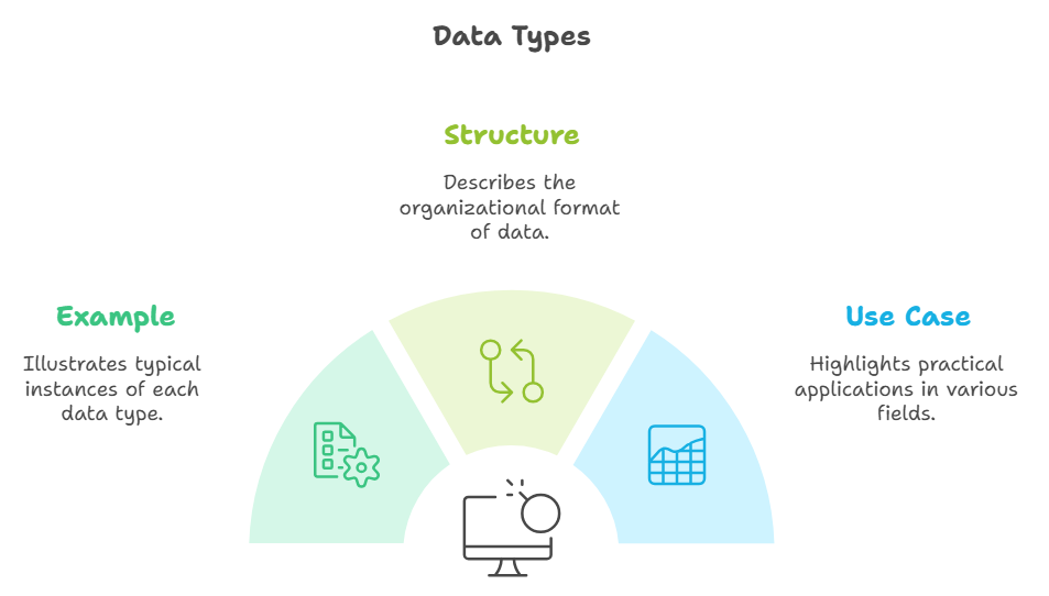
Feature	Rectangular Data	Non-Rectangular Data
Example	Customer data table	Time series, spatial data, graph data
Structure	Rows and columns	More complex structures like networks
Use Case	Business analytics, ML models	IoT, location analytics, recommender systems

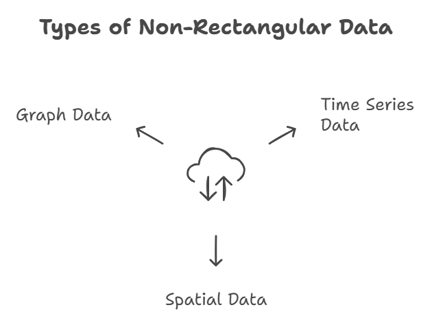
Non-Rectangular Data Structures

Time Series Data: A collection of measurements taken over time, showing how variables change. It is essential for IoT.
Spatial Data: Used for mapping and location analytics, e.g., GIS systems.
Graph Data: Represents relationships, such as social networks or physical hubs connected by roads.

Example for Corporate Employees: Recommender systems like Amazon's "Customers also bought" use graph data structures.

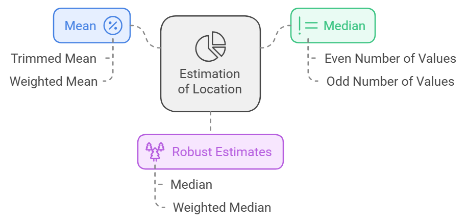
Estimation of Location

Finding the central tendency is key when analyzing variables with many distinct values.

Mean

The mean is the sum of all values divided by the number of values.
Example: {3, 2, 5, 1} → Mean = (3+2+5+1) / 4 = 2.75

Trimmed Mean

Removes extreme values from the start and end before calculating the mean.
When there is a competition going on, 10 judges are there we can remove 2% from the start and end so remaining will be 6 judges and we will consider their marks so that bias gets removed.
Example Formula:

$$\text{Trimmed Mean} = \frac{1}{n - 2p} \sum_{i=p+1}^{n-p} x_{(i)}$$

Use Case: Helps when extreme values (outliers) may skew results. When you draw the distribution of the results there will be skewness in the distribution. Trimmed Means will help to reduce that skewness.

Weighted Mean

Multiplies each value by its weight before calculating the mean.

The weighted mean gives more importance to some values than others, which is useful when certain data points carry more weight or significance

$$\text{Weighted Mean} = \frac{\sum_{i=1}^{n} w_i x_i}{\sum_{i=1}^{n} w_i}$$
Use Case: Helps adjust for underrepresented or overrepresented groups in a dataset.

Median and Robust Estimates

Median: The centre value of sorted data.
If the number of values is even, it is the average of the middle two values.
Weighted median adjusts for weights assigned to each data point.

Tip: Both median and weighted median are robust to outliers, making them better estimates for central tendency in skewed datasets.

Outliers

Outliers are values distant from the majority of data points.
They can result from data errors (e.g., mixed units or sensor issues) or genuine anomalies.
Outliers may not always be errors; they can hold valuable information.

Call to Action:
Have you encountered outliers in your dataset? Analyze the given Murder Rates by States dataset using the techniques discussed here.

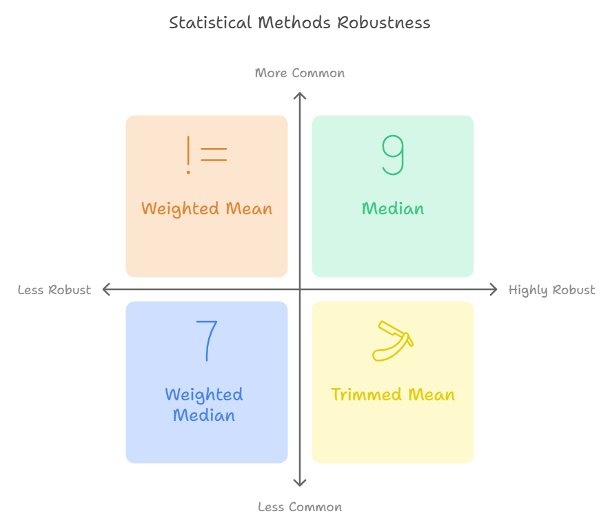
Rankings for Robustness

Rank	Method	Robustness to Outliers
1	Median	Highly robust
2	Weighted Median	Highly robust
3	Trimmed Mean	Moderately robust
4	Weighted Mean	Less robust

Practical Implementation

Use Python libraries for practical implementation:
- Mean and Median: pandas
- Weighted Mean: NumPy
- Weighted Median: wquantiles
- Trimmed Mean: scipy.stats

import pandas as pd
import numpy as np
import scipy.stats as stats
import wquantiles

# Sample DataFrame
data = pd.DataFrame({
    "Values": [3, 2, 5, 1, 100],
    "Weights": [1, 1, 1, 1, 2]
})

# Mean and Median
mean = data["Values"].mean()
median = data["Values"].median()

# Weighted Mean using NumPy
weighted_mean = np.average(data["Values"], weights=data["Weights"])

# Weighted Median using wquantiles
weighted_median = wquantiles.median(data["Values"], data["Weights"])

# Trimmed Mean using scipy.stats
trimmed_mean = stats.trim_mean(data["Values"], proportiontocut=0.2)

# Display results
print(f"Mean: {mean}, Median: {median}")
print(f"Weighted Mean: {weighted_mean}, Weighted Median: {weighted_median}")
print(f"Trimmed Mean: {trimmed_mean}")

Final Thoughts

By this time you need to get to know about one of the procedures in EDA which is an estimation of location as well as what are better methods to do an estimation of location and also what modules you need to use to estimate the locations. Understanding data structures and measures of location is crucial for data science. Whether you’re a student building projects or a corporate employee analyzing business data, mastering these basics will help you make informed decisions.

If you want to learn more buy Practical Statistics for Data Scientists: 50 Essential Concepts by Andrew Bruce and Peter Bruce

Apply these concepts to real-world datasets and enhance your skills. Share your findings in the comments!

Practical Data Science: Rectangular Data and Estimation Techniques