Overview

I developed an image-sharing API that allows authenticated users to upload images, which can be viewed by other authenticated users following them within the app. One requirement for this API was to integrate AI-based image classification, categorizing uploaded images into four main groups.

The image categories for this app are Nature, Sports, Architecture, and Fashion. The primary objective of integrating AI is to automatically analyze images uploaded by users and assign each image to one of these predefined categories based on a trained machine learning model.

However, a key question for this AI integration is: what happens when an uploaded image doesn’t fit into any of the specified categories? For example, if a user uploads a picture of a product in a grocery store aisle, this image could potentially fit into Nature or Architecture, depending on interpretation. Similarly, an image of a pilot flying a plane could be classified as either Nature or Sports, and a photo of people dressed up and dancing might be considered Sports or Fashion.

At this stage, we can’t do much about ambiguous cases within this tutorial. The model we train here will assign each image to the category it determines to be the best fit based on the data it was trained on. Over time, refining the model with more diverse data could help improve its accuracy in distinguishing these subtleties.

Prerequisite

A solid understanding of Python and API development in Python is necessary to follow this tutorial smoothly.
I'm using a Mac for development, so all the provided commands are Mac-specific.
You'll also need accounts on Google and Hugging Face. Make sure you've created and copied your API keys for authenticating deployments on Hugging Face.
Review the project notebook files
1. image_classification_training.pynb
2. image_classification_inference.pynb

Tools and Software Used

The following are core technologies that I adopted for this project.

Fastai

Fastai is a deep learning library built on top of PyTorch that simplifies building, training, and fine-tuning models for tasks like image classification, natural language processing, and tabular data analysis. In this project, we used Fastai to leverage pre-trained models and its high-level APIs to quickly set up an image classifier, enabling the application to classify user-uploaded images into specific categories.

Google Colab

Google Colab is a cloud-based platform that offers free access to GPU-powered Jupyter notebooks, making it ideal for running computationally intensive machine learning experiments. We used Google Colab to prototype and train the image classification model in an interactive environment, taking advantage of its GPU support to speed up model training without needing local hardware resources.

Hugging Face

Hugging Face is a platform and open-source library for natural language processing and machine learning that includes model hosting, deployment, and various NLP tools. We used Hugging Face to host the trained model, making it accessible for the API to integrate image classification functionalities without directly handling model deployment and management on our end.

Gradio

Gradio is a Python library that allows you to build web-based interfaces for machine learning models, enabling users to interact with models directly from a browser. In our project, Gradio was used to create an interface where users can upload images and see the classification results in real time, providing an interactive way to test and showcase the capabilities of your image classifier. Gradio also enables us to access the hosted model as an API which is the core functionality we need to send image analysis requests from the image-sharing API.

The Development

Getting Set

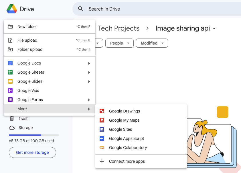
Open your project folder in your Google Drive and click on +New and hover on More to show the sub-menu. Click on Google Colaboratory.

Rename the notebook that has been created from ‘untitled’ to the name of the project.

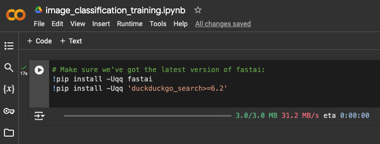
In the first code cell, install the required packages for the project.

Gathering Data

The success of a model largely depends on the quality of images used for training. The model we are developing would only be able to classify images into the defined categories if it was trained with a wide variety of data to cover various perspectives of what these categories could look like. This classifier, needs a diverse set of images of nature, sports, architecture and fashion. But where can we obtain this data?

For this project, we will download these images from the web using the Duckduckgo browser. This approach carries some risk, as we cannot fully control the types of nature, sports, architecture and fashion images available online. An ideal approach for training data collection would involve curating a large, high-quality dataset of images featuring nature, sports, architecture and fashion. However, this could become quite costly, as it would require collaboration with other project contributors to source these images.

Images used in training the model should be closely related to the type of images the model will be given to analyse in the production environment. Structural or style differences in the training data may make the model perform poorly in production.

Downloading Training Images

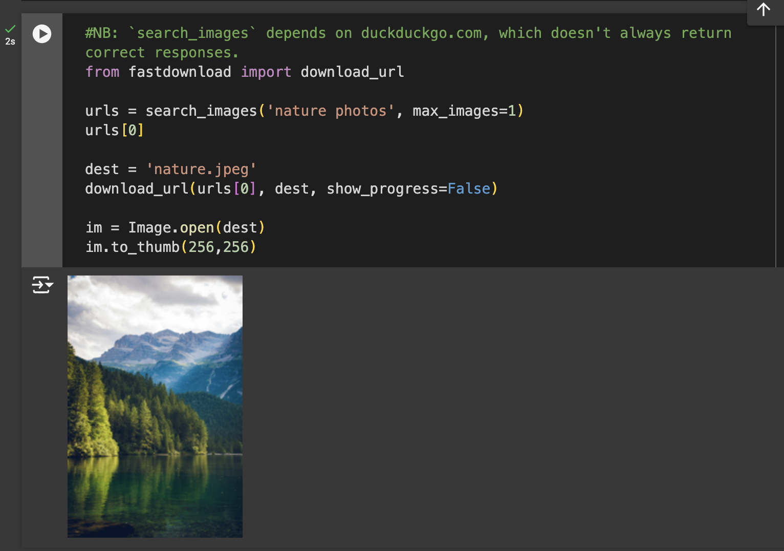
Let's start by searching for an image of nature to examine the type of images we can retrieve. The cell below uses the search_images function to download 200 URLs as a result of the search keywords on the Duckduckgo browser.

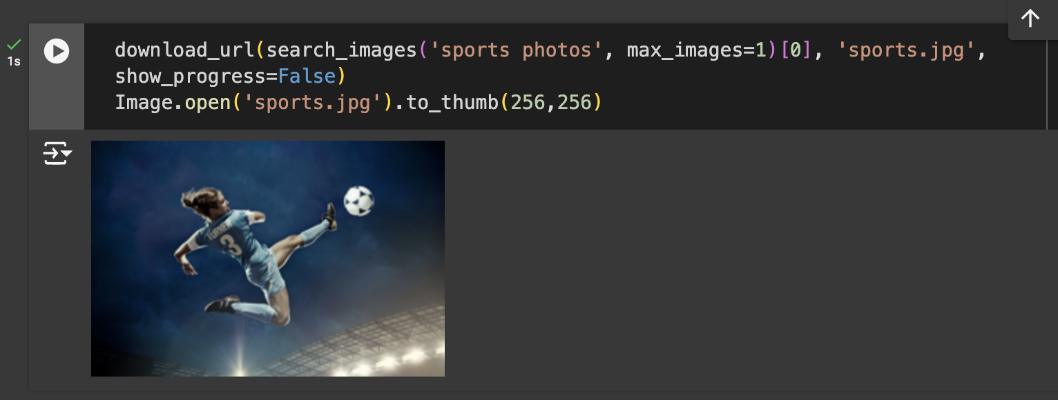
On cells 3 and 4, to get a sense of the type of images we can obtain, we carry out a test for downloading a single nature and sports image using the function.

Since the images we could obtain online are satisfactory to a fair degree, we can proceed to the next cell. Cell 5 automates the process of creating folders for each image category (Nature, Sports, Architecture, Fashion), downloading relevant images for each category, and resizing them to a standard size. It uses a loop to search for images based on each category, creates the necessary directory if it doesn’t already exist, and then saves and resizes the images into their respective folders. We now have a total of a maximum of 800 images across the four categories. View the newly created files in the project folder.

In the following cell, we check the downloaded images for any files that might be corrupted. Any invalid images are removed to ensure our dataset remains clean, and we then count how many files were deleted.

Training the Model

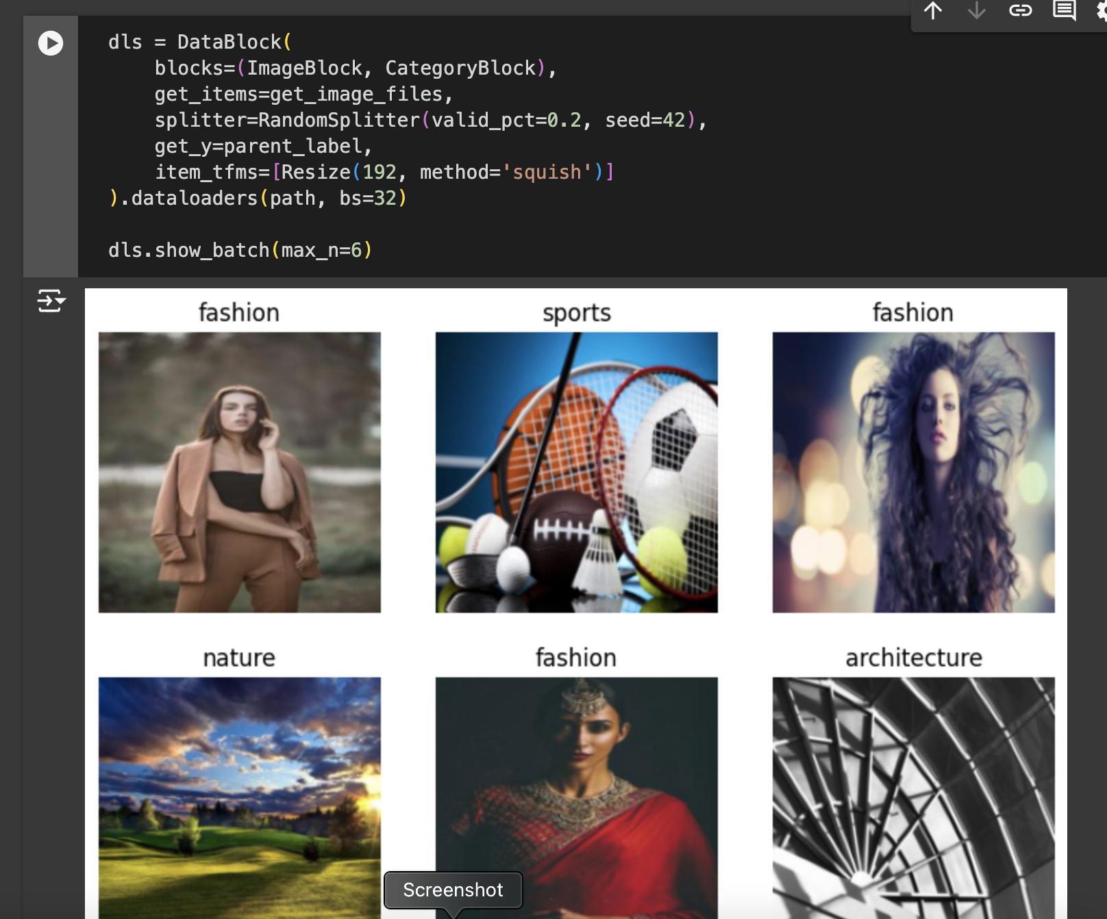
dls = DataBlock(...): This line initializes a DataBlock, which is a flexible class in Fastai that helps in setting up the data pipeline by specifying how data should be loaded, transformed, and split. Fastai requires four key details to create DataLoaders:
- What types of data it should work with (e.g., images and labels)
- How to retrieve or get the items (e.g., loading images from a directory)
- How to split the data into training and validation sets
- How to label or get the “y” values (dependent variable)
blocks=(ImageBlock, CategoryBlock): This defines the types of data we’re working with in DataBlock. ImageBlock represents our independent variable (X) or inputs—image files in this case—while CategoryBlock represents our dependent variable (y) or labels, which are the categories we want the model to predict.
get_items=get_image_files: This specifies how to retrieve the images. get_image_files is a Fastai utility that finds all image files within a given path, helping us load the data.
splitter=RandomSplitter(valid_pct=0.2, seed=42): This sets how to split the data into training and validation sets. Here, RandomSplitter is used to randomly allocate 20% of the data as a validation set. By using seed=42, we ensure the split is reproducible, so the same images are always in the validation set, which is essential for consistency when training and testing.
get_y=parent_label: This tells Fastai how to label each image. parent_label grabs the name of the parent folder as the label (category), assuming each category of images is stored in a separate folder named accordingly.
item_tfms=[Resize(192, method='squish')]: This applies a transformation to each image, resizing it to 192x192 pixels using the squish method. Fastai offers different resizing approaches:
- Crop: crops the image to fit the desired dimensions, potentially cutting out parts of the image.
- Pad: adds padding to maintain the aspect ratio, potentially adding blank areas.
- Squish: resizes by stretching or compressing without preserving the original aspect ratio, which is fast but can distort images.
- Choosing between these depends on the use case: crop or pad is preferred for preserving image content and proportion, while squish is useful for simplicity and computational efficiency.
.dataloaders(path, bs=32): This finalizes the data pipeline by creating DataLoaders from the DataBlock. DataLoaders is a Fastai object that loads the data in batches (sets of images) for training and validation, using a batch size (bs) of 32.
dls.show_batch(max_n=6): This displays a sample of 6 images with their respective labels from the data, giving a quick visual confirmation of the data preparation and transformations applied.

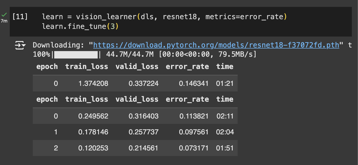
This cell sets up and trains a deep-learning model using Fastai’s vision_learner function. Here, resnet18 is the chosen architecture—a popular convolutional neural network (CNN) model that has been pre-trained on a large dataset, allowing it to recognize common visual patterns. By passing resnet18 to vision_learner, we leverage this pre-trained model, which speeds up training and often improves accuracy.

The fine_tune(3) function then refines the model specifically for our image categories. Fine-tuning adjusts the pre-trained weights to better fit our dataset by unfreezing the last layers first and training for 3 epochs, effectively customizing it for our classification task. The error_rate metric tracks the model's performance, helping us evaluate and monitor improvements during training.

Cleaning the Data

What is a confusion matrix? A confusion matrix shows us the mistakes the model is making.

The rows represent all the nature, sports, architecture and fashion images in our dataset, respectively. The columns represent the images which the model predicted as nature, sports, architecture and fashion images, respectively. Therefore, the diagonal of the matrix shows the images which were classified correctly, and the off-diagonal cells represent those which were classified incorrectly.

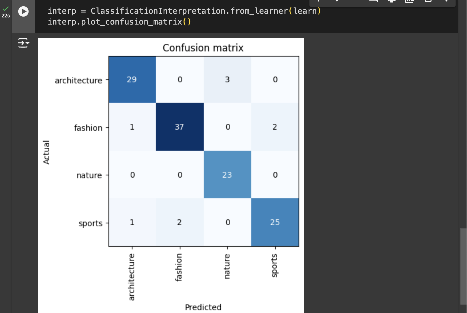
Architecture: 29 images were correctly classified as Architecture, but 3 were misclassified as Nature.
Fashion: 37 images were correctly classified, with 1 misclassified as Architecture and 2 as Sports.
Nature: All 23 Nature images were correctly classified.
Sports: 25 images were correctly classified, with 1 misclassified as Architecture and 2 as Fashion.

This matrix shows that while the model performs well in most categories, there is some confusion, especially between similar or overlapping categories, such as Fashion and Sports.

The interp.plot_top_losses(5, nrows=1, figsize=(17,4)) command visualizes the five images that the model misclassified with the highest confidence, giving insight into where the model struggles most.

interp.plot_top_losses(5, ...): This function from Fastai's ClassificationInterpretation class displays the top 5 errors (highest loss) that the model made. "Top losses" refer to cases where the model was most incorrect and most confident, which often reveals challenging or ambiguous images.
nrows=1: This arranges the images in a single row for a clearer, side-by-side view.
figsize=(17,4): This sets the overall dimensions of the plot to 17 inches wide by 4 inches tall, giving each image enough space to be visible.

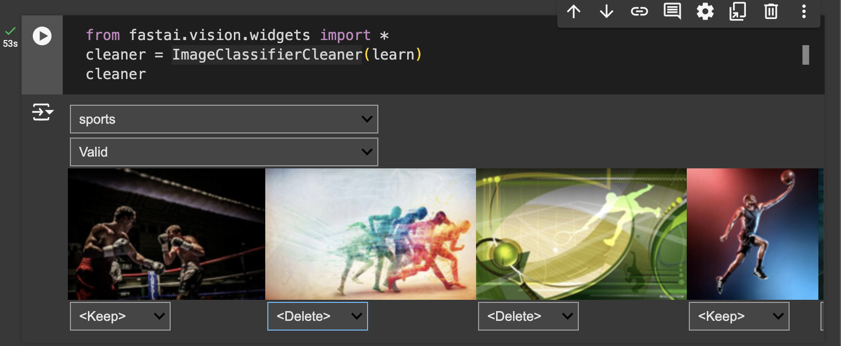
This cell sets up an interactive tool to help us clean and refine our dataset.

ImageClassifierCleaner(learn): This widget from Fastai creates an interface for reviewing model predictions. It displays images that may have been misclassified or ambiguous, letting us easily identify and reassign categories or delete incorrect images.
cleaner: By simply running cleaner, we bring up the interactive tool in the notebook.

This widget is particularly helpful for improving the quality of our dataset by allowing us to correct labels and remove mislabeled or poor-quality images without manually searching through the files.

For each of the data categories we are working with, we can review the images for both the training and the validation data manually to assess whether they are suitable for the category. If necessary, we can delete the image or assign it to a more suitable category.

This cell deletes images from the dataset marked for removal using the ImageClassifierCleaner widget.

for idx in cleaner.delete(): This part loops through the indices of images flagged for deletion in the cleaner interface.
cleaner.fns[idx].unlink(): For each flagged image, unlink() removes the file from the dataset, permanently deleting it from the filesystem.

This step helps us quickly and efficiently clean up any irrelevant or incorrect images, improving the overall quality of the training data for future model training.

Test Model Predictions

Export the Trained Model

As a final step in our model training notebook, we need to export the model.pkl file.

What is model.plk ? The model.pkl file is a saved version of our trained model, stored in a format that can be easily reloaded for later use.

learn.export('model.pkl'): This command saves the entire model, including its architecture, learned parameters, and any custom settings, into a file called model.pkl. This makes it possible to deploy or share the model without needing to retrain it each time, which saves time and computational resources.

Exporting the model in this way is essential for real-world applications, as it allows us to use the trained model directly in production environments or load it into another project for further analysis or development.

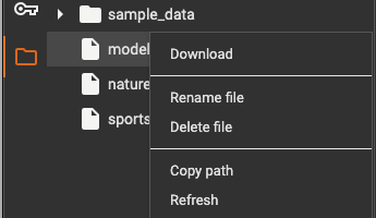
In the project runtime directory in Google Colab, click on Download to download the model.pkl file to your local PC.

Inference

Inference refers to when we use the model for getting predictions, instead of training.

We are going to use a separate notebook on Google Colab to use our trained model to make predictions. Start a new notebook as we have previously demonstrated in your preferred folder. You can name it image_classification_inference.ipynb

This full notebook file can be found here

In the first cell adding # | default_exp app at the top of a Fastai notebook designates the default module name (in this case, app) for the code written in the notebook. This allows Fastai's nbdev tool to automatically organize and export the notebook code into a Python script named app.py, making it easier to package and reuse the code outside the notebook.

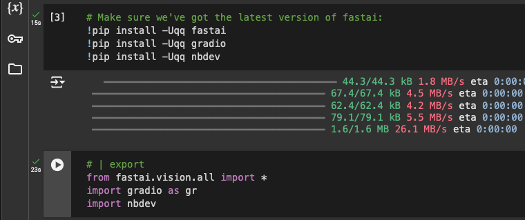
Then project dependencies are installed and imported in the following cells.

In the project’s content directory, we upload an image to use for testing the model. The following cell retrieves this image file from the content directory, resizes it to a thumbnail, and displays it for review.

This cell code will create a PIL image from the file, resize it to 192x192 pixels for easier viewing, and return the processed image.

To create our inference learner from the exported file, we use load_learner. The model.pkl file that we downloaded at the end of the model training notebook must be uploaded in the content directory.

To classify a single image, we pass its filename to the model's predict function. In this example, the model correctly predicted the image as belonging to the "nature" category.

The output provides three pieces of information: the predicted category label ("nature"), the corresponding tensor index for that category (tensor(2)), and a tensor of confidence scores for each category. The confidence scores indicate the model's certainty, with a 97.4% probability assigned to "nature," showing strong confidence in this classification.

learn.dls.vocab returns a list of the categories for the predictions from the trained model. classify_image(img) function takes an image (img) as input and uses the model to predict its category.
- learn.predict(img): This method generates the prediction for the input image. It returns the predicted label (pred), the index of that label (idx), and a tensor of probabilities (probs) for each category.
- dict(zip(categories, map(float,probs))): This line creates a dictionary that pairs each category with its corresponding confidence score (converted to a float) from probs, allowing for an easy-to-read output of confidence levels for each category.

The classify_image function returns a dictionary showing the model’s confidence for each category, which is useful for understanding how strongly the model predicts the image’s classification.

In this cell, we use Gradio to create a web interface that lets users interact with the trained model for real-time predictions. Upload example images for each category into the project’s content directory to test the model directly from the interface.
- Line 2 (image = gr.Image(type='pil')): Sets the input to be an uploaded image, which will be processed in PIL format to ensure compatibility with the model.
- Line 3 (label = gr.Label()): Specifies that the output will be a label showing the model's predicted category.

The demo variable creates an interactive Gradio interface with classify_image as the main function, using image as input and label as output. Clicking the link generated by demo.launch() opens the web interface, where users can upload images to see the model’s predictions along with confidence scores.

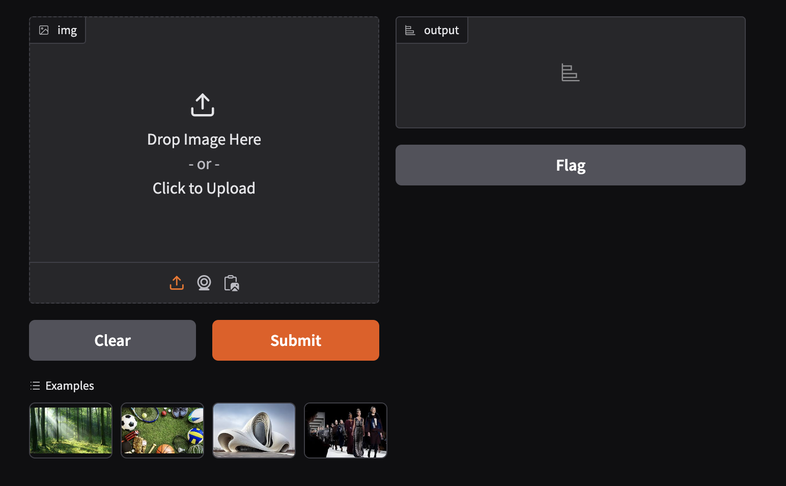
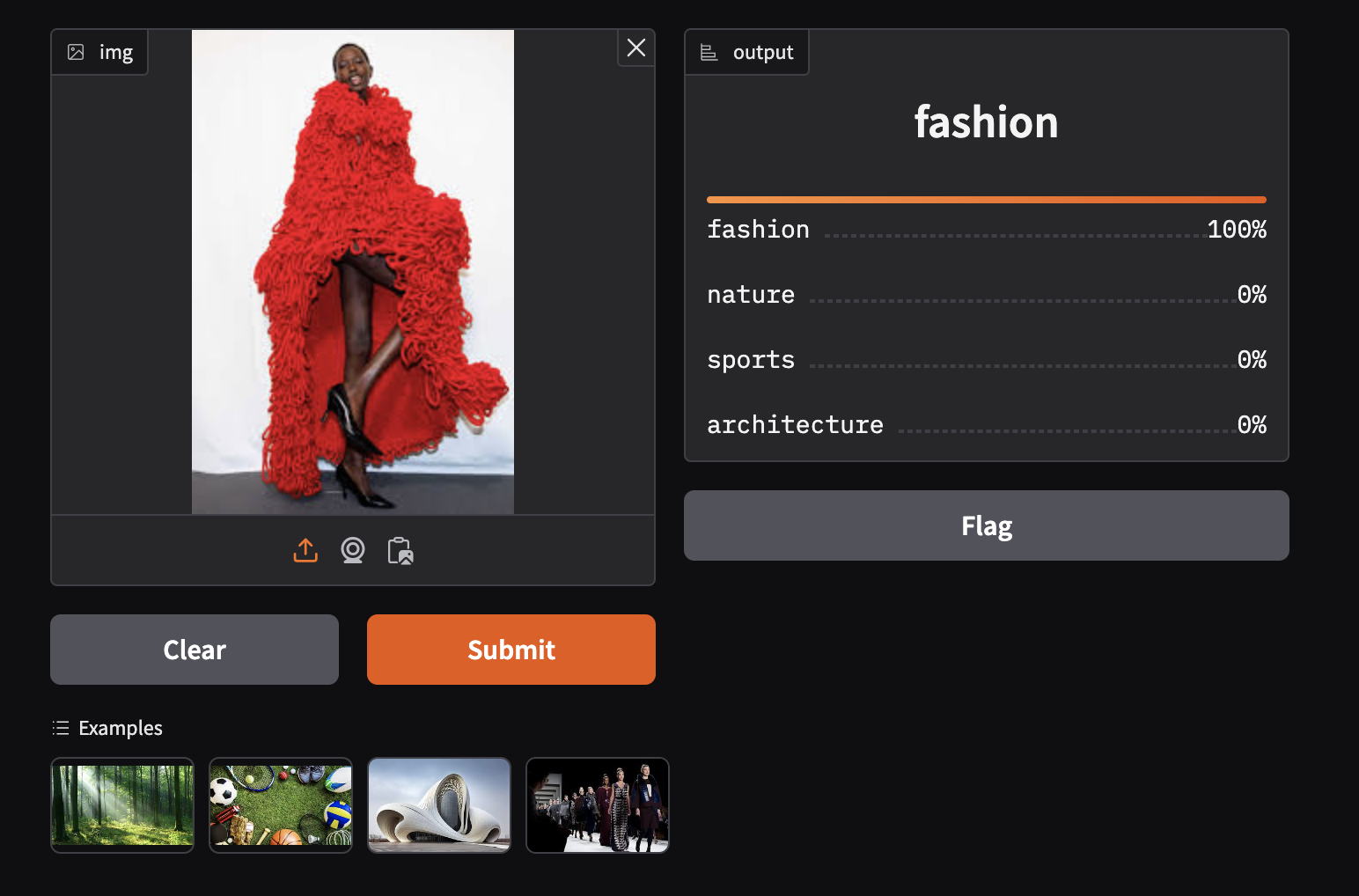
Here we upload an image of a woman wearing a fashionable clothing piece and the model accurately predicts the image category as fashion.

In another test we upload an image obtained from a google search for architecture and as you can see, the model wronly classifies this as a nature image. Understandly so.

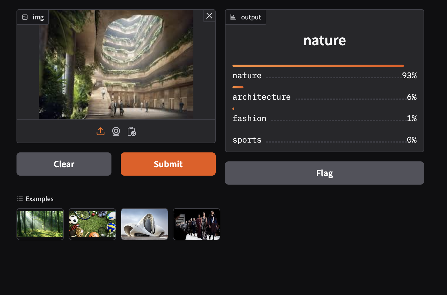
The final cell in this notebook exports tagged code cells as a Python script, app.py which is saved in the project’s content directory and can be downloaded to your local pc. This process isolates the essential code needed to run the model independently as a Python script.

By specifying the notebook filename and export location, nbdev.export.nb_export converts the notebook into a streamlined .py file, making it ready for use in production or as a standalone script to load and interact with the model.

Create a Web App for the Model

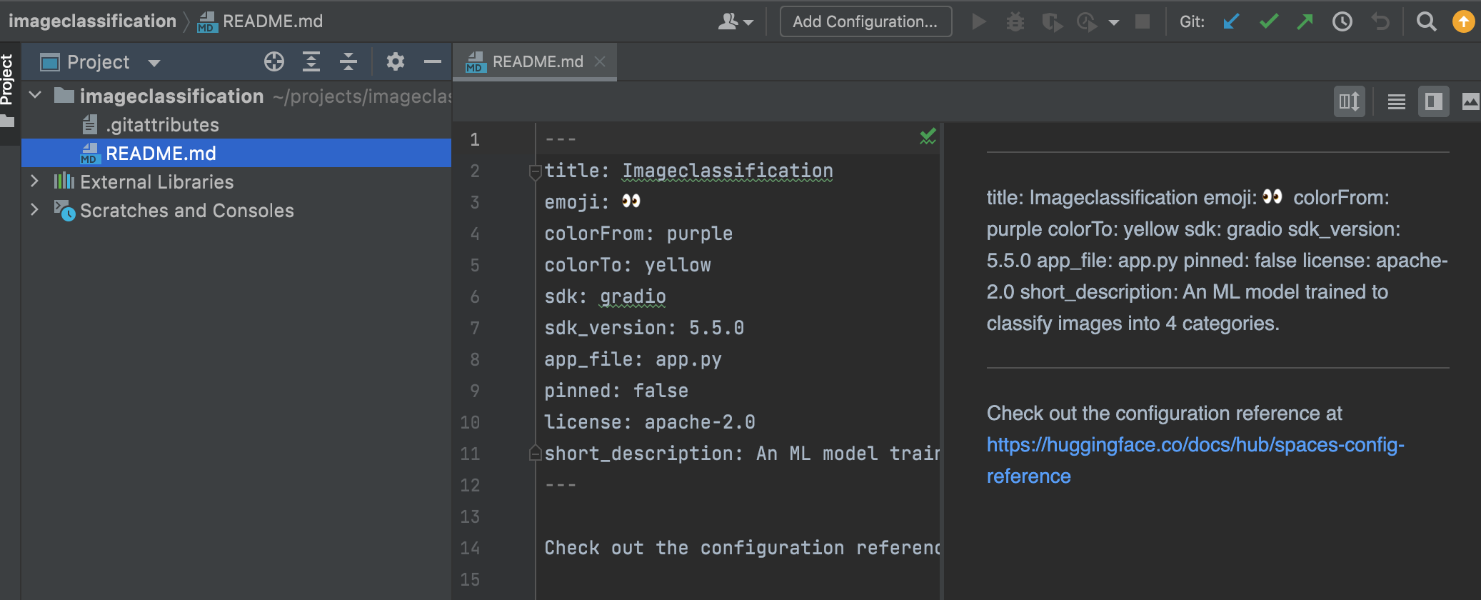
Set Up Hugging Face Space

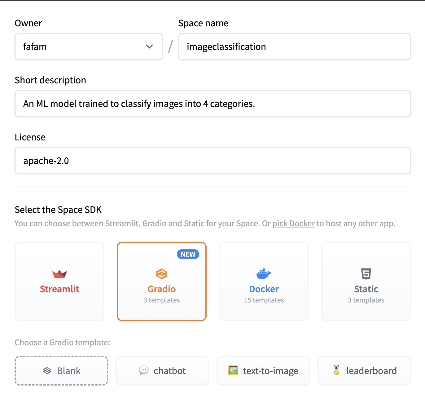
Open Hugging Face Spaces page and click Create New Space.

Give the space a name and a short description. Select a suitable license. Select Gradio as a space SDK and leave the preselected blank Gradio template.

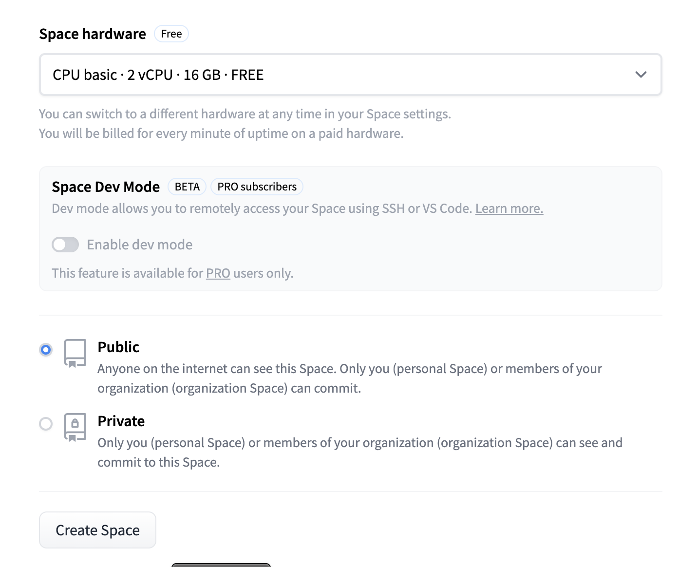
Use the free CPU Basic hardware and leave the space Public. click Create space.

Deploy the model to Hugging Face

Use the command displayed when the space is set up to clone the space to your local PC. When prompted for a password, use an access token with write permissions. Generate one from your settings: https://huggingface.co/settings/tokens

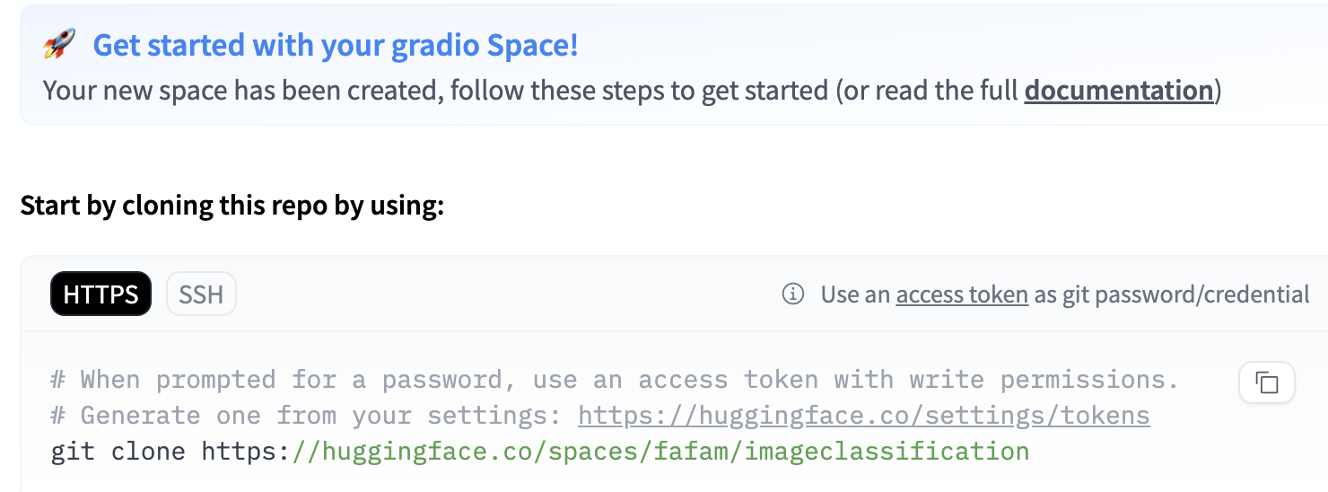
Open the project folder in your preferred programming IDE. I am using PyCharm.

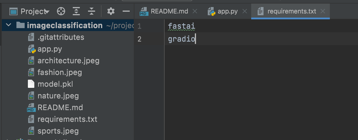
update the project directory with the following files:
- model.pkl file we used to train the model.
- app.py file we downloaded after testing the model on a notebook.

    # AUTOGENERATED! DO NOT EDIT! File to edit: image_classification_inference.ipynb.

    # %% auto 0
    __all__ = ['learn', 'categories', 'image', 'label', 'examples', 'demo', 'classify_image']

    # %% image_classification_inference.ipynb 2
    from fastai.vision.all import *
    import gradio as gr

    # %% image_classification_inference.ipynb 4
    learn = load_learner('model.pkl')

    # %% image_classification_inference.ipynb 6
    categories = learn.dls.vocab

    def classify_image(img):
        pred,idx,probs = learn.predict(img)
        return dict(zip(categories, map(float,probs)))

    # %% image_classification_inference.ipynb 8
    image = gr.Image(type='pil')
    label = gr.Label()
    examples = ['nature.jpeg', 'sports.jpeg', 'architecture.jpeg', 'fashion.jpeg']

    demo = gr.Interface(fn=classify_image, inputs=image, outputs=label, examples=examples)
    demo.launch(inline=False)

requirements.txt file with the project dependencies

    fastai
    gradio

The 4 example images to support a user with reference images for classification.

Use the commands below to add the new files to git, commit them and push them to the space. ensure that you are authenticated properly to carry out this action.
```
  git add app.py requirements.txt nature.jpeg architecture.jpeg sports.jpeg fashion.jpeg
  git commit -m "initial commit"
  git push
```
Your model is now successfully deployed as a web app that can be accessed from anywhere using the URL https://huggingface.co/spaces/fafam/imageclassification

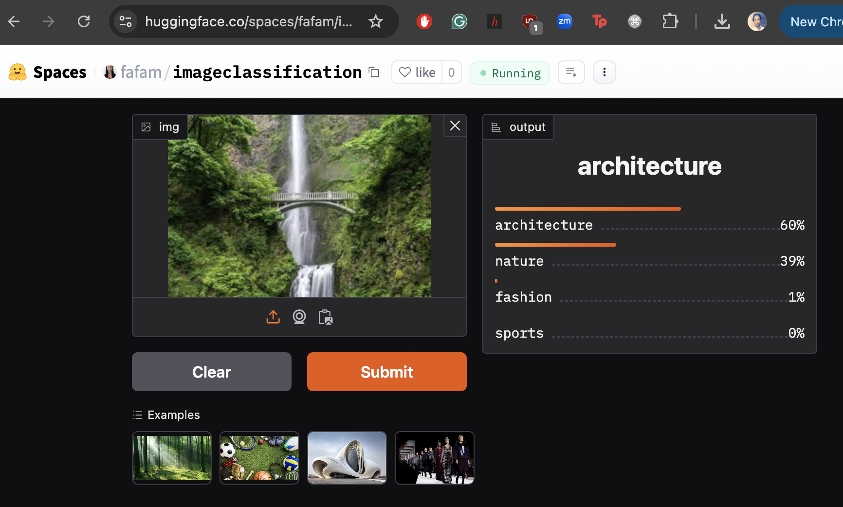
I tested the model again using an image I obtained from the results of a Google image search for “nature” and as you can see, our model has classified this under architecture. :) :D

Using the Model in Production

Gradio allows us to access the model we have just deployed on production via an API. At the bottom of the web app, is a link to read instructions on accessing the model via an API.

Test model in Django web API app

We are going to use the classifier model we have trained in a Django web API app for categorising image posts that a user uploads across the 4 categories (Nature, Sports, Architecture, and Fashion).

Install the required dependencies in the project virtual environment.

pip install gradio_client

In the project folder, we create a new Python file called imageclassifier.py and update it with the following code.

import tempfile
from gradio_client import Client, handle_file

client = Client("fafam/imageclassification")


def classify_image(image):
    # Save the PIL image to a temporary file
    with tempfile.NamedTemporaryFile(suffix=".jpeg", delete=True) as temp_file:
        image.save(temp_file, format="JPEG")  # Save the image in an appropriate format
        temp_file.flush()  # Ensure all data is written to the file

        # Pass the temporary file's path to handle_file
        result = client.predict(
            img=handle_file(temp_file.name),
            api_name="/predict",
        )
    return result

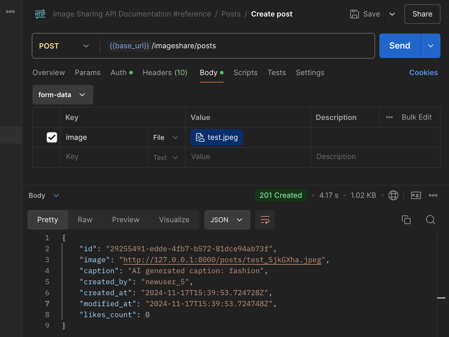
You can review the source code for our example Django web app for image sharing here. The app incorporates AI-powered image classification when a user uploads an image. Our trained machine learning model classifies the uploaded image into one of four categories and returns a label, which is then used as the AI-generated caption for the image.


class PostViewSet(viewsets.ModelViewSet):

    serializer_class = PostSerializer
    permission_classes = [permissions.IsAuthenticated]
    pagination_class = PostsPagination
    filter_backends = [filters.SearchFilter]  # Add search filter backend
    search_fields = ["caption"]  # Specify fields for search

    def perform_create(self, serializer):
        # Retrieve the image file from the request
        image_file = self.request.FILES.get('image')

        if image_file:
            # Open the in-memory image file
            image = Image.open(image_file)

            # Call classify_image with the opened image or its content
            ai_caption = classify_image(image)['label']

            # Save the serializer with the additional ai_caption and user
            serializer.save(created_by=self.request.user,
                            caption=f"AI generated caption: {ai_caption}"
                            )
        else:
            raise ParseError("No image file provided.")

The code defines a PostViewSet, which is responsible for handling user interactions with posts in the application. The perform_create method is customized to incorporate image classification functionality, enhancing the user experience by automatically generating a caption for uploaded images. Here's a breakdown of how it works:
1. User Uploads an Image: When a user submits a POST request to create a new post, they must include an image file in their request. The uploaded file is retrieved using self.request.FILES.get('image').
2. Image Processing: The uploaded file is opened in-memory using the Python Imaging Library (PIL). This step ensures the image is prepared for further processing.
3. Integration with an ML Model: The image is passed to the classify_image function, which sends a request to a pre-trained machine learning model hosted on Hugging Face. The function interacts with the model's API endpoint and returns a classification result in JSON format.
4. Generating an AI-Based Caption: The classification result includes a label corresponding to the predicted category of the uploaded image. This label is extracted from the response and used to generate a caption for the post, prefixed with "AI generated caption:" to distinguish it as AI-derived.
The response to the request is below

Conclusion

Areas for Improvement and Considerations for Model Enhancement

Data Quality and Representation

One critical area for improvement is the quality and diversity of the training data. For the model to perform effectively, the dataset must accurately represent the full range of variations within each category. Currently, there is a risk that the model may fail to recognize images that deviate from the patterns it has been trained on. For instance, variations in lighting, perspective, or context within the images may lead to misclassification or failure to classify altogether. Enhancing the dataset by including diverse and contextually rich examples for each category would help the model generalize better and improve its performance in real-world scenarios.

Handling Edge Cases and Out-of-Category Inputs

Another key consideration is how the model handles inputs that fall outside the defined categories. For example, if the model is presented with an image of a student celebrating their graduation—an event that doesn’t belong to any of the pre-defined categories—it may struggle to provide a meaningful output. This could result in:

Misclassification: The model might incorrectly assign the image to one of the existing categories, leading to inaccurate results.
Failure to Classify: Depending on the implementation, the model might return a default or null value, which may not be useful.

To address such scenarios, several strategies can be employed:

Introduce an "Unknown" Category: Extend the model's training to include an "Unknown" or "Other" category, populated with a diverse range of images that do not belong to the core categories.
Confidence Thresholding: Implement a confidence scoring mechanism. If the model's prediction confidence falls below a certain threshold, the image can be flagged as "Unclassifiable" or require manual review.
Out-of-Distribution Detection: Use techniques like anomaly detection to identify inputs that significantly deviate from the training distribution, allowing the system to handle such cases appropriately.

Build an ML Model for Classifying Images in a Django API App using Fastai, Hugging Face, Gradio and Colab

Table of contents