Seasonality is a fundamental concept in time series analysis and forecasting. It refers to periodic fluctuations that occur at regular intervals due to seasonal factors. Understanding seasonality is crucial for accurate forecasting and making informed decisions based on time series data.

What is Seasonality?
Importance of Seasonality in Time Series Analysis
Types of Seasonality
- Additive Seasonality
- Multiplicative Seasonality
Identifying Seasonality
Modeling Seasonality
Handling Seasonality in Forecasting
- Deseasonalizing Data
- Incorporating Seasonality into Models
Practical Implementation with Python
Conclusion

What is Seasonality?

Seasonality in time series data refers to patterns that repeat over known, fixed periods due to seasonal factors. These patterns can be influenced by:

Climate Seasons: Changes in weather affecting sales of seasonal products.
Calendar Effects: Holidays, weekends, or specific dates influencing consumer behavior.
Business Cycles: Quarterly financial reporting leading to predictable fluctuations.

Characteristics of Seasonality:

Regular Intervals: Occurs at consistent periods (daily, weekly, monthly, quarterly, annually).
Predictable Patterns: The fluctuations can be anticipated based on historical data.
Influenced by External Factors: Often driven by factors outside the time series itself.

Importance of Seasonality in Time Series Analysis

Understanding and accounting for seasonality is crucial for several reasons:

Improved Forecast Accuracy: Models that incorporate seasonality can make more accurate predictions.
Resource Planning: Businesses can plan inventory, staffing, and budgeting around seasonal peaks and troughs.
Identifying True Trends: Removing seasonal effects helps in identifying underlying trends and patterns.

Types of Seasonality

Seasonality can manifest in different ways in time series data, primarily classified into Additive and Multiplicative seasonality.

Additive Seasonality

Definition: Seasonal fluctuations are constant over time.
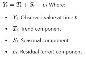
Mathematical Representation:
When to Use: When the magnitude of seasonal variations does not depend on the level of the time series.

Multiplicative Seasonality

Definition: Seasonal fluctuations change proportionally with the level of the time series.
Mathematical Representation:
When to Use: When the magnitude of seasonal variations increases or decreases with the level of the series.

Identifying Seasonality

Visual Inspection

Plotting the time series is the first step in identifying seasonality.

Line Plots: Observe repeating patterns over fixed periods.
Seasonal Plots: Plot data for each season separately to compare patterns.
Box Plots: Use box plots to visualize distribution across seasons.

Autocorrelation Function (ACF) and Partial Autocorrelation Function (PACF)

ACF: Measures correlation between observations at different lags.
PACF: Measures the partial correlation at different lags after removing effects of earlier lags.
Seasonal Lags: Significant spikes at seasonal lags indicate seasonality.

Seasonal Decomposition

Purpose: Decompose the time series into trend, seasonal, and residual components.
Methods:
- Additive Decomposition
- Multiplicative Decomposition
Tools: Use statistical software or libraries (e.g., statsmodels in Python) for decomposition.

Modeling Seasonality

Seasonal ARIMA Models

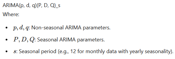
SARIMA: Seasonal AutoRegressive Integrated Moving Average.
Incorporates: Both non-seasonal and seasonal factors in the ARIMA model.
Model Notation:

Exponential Smoothing Methods

Holt-Winters Method: Extends simple exponential smoothing to capture trend and seasonality.
Types:
- Additive Seasonality: For constant seasonal variations.
- Multiplicative Seasonality: For proportional seasonal variations.

Seasonal Decomposition of Time Series (STL)

STL Decomposition: Seasonal-Trend Decomposition using Loess (Locally Estimated Scatterplot Smoothing).
Advantages:
- Handles any type of seasonality.
- Robust to outliers.
Applications: Used for exploratory analysis and preprocessing.

Handling Seasonality in Forecasting

Deseasonalizing Data

Purpose: Remove seasonal effects to analyze the underlying trend and cyclical components.
Process:
- Calculate Seasonal Indices: Average the data for each season.
- Adjust Data:
  - Additive Model: Subtract seasonal indices.
  - Multiplicative Model: Divide by seasonal indices.

Incorporating Seasonality into Models

Include Seasonal Terms: Add seasonal variables or lags in regression models.
Use Seasonal Models: Employ models designed to handle seasonality (e.g., SARIMA, Holt-Winters).

Practical Implementation with Python

Let's apply these concepts using Python libraries such as pandas, numpy, matplotlib, statsmodels, and seaborn.

Data Preparation

We'll use a sample dataset to illustrate seasonality.

import numpy as np
import pandas as pd
import matplotlib.pyplot as plt
import seaborn as sns

# For time series analysis
from statsmodels.tsa.seasonal import seasonal_decompose
from statsmodels.graphics.tsaplots import plot_acf
from statsmodels.tsa.statespace.sarimax import SARIMAX

# Generate synthetic time series data with seasonality
np.random.seed(0)
periods = 48  # Monthly data for 4 years
time = pd.date_range(start='2018-01-01', periods=periods, freq='M')

# Create seasonal pattern
seasonal_pattern = [10, 12, 15, 20, 25, 30, 25, 20, 15, 12, 10, 8] * 4

# Create trend
trend = np.linspace(50, 100, periods)

# Combine components with some noise
data = trend + seasonal_pattern + np.random.normal(scale=5, size=periods)

# Create DataFrame
df = pd.DataFrame({'Date': time, 'Value': data}).set_index('Date')

Visualizing Seasonality

Line Plot

plt.figure(figsize=(12, 6))
plt.plot(df.index, df['Value'], marker='o')
plt.title('Time Series Data')
plt.xlabel('Date')
plt.ylabel('Value')
plt.grid(True)
plt.show()

Seasonal Plot

# Extract month from the date
df['Month'] = df.index.month

# Boxplot to visualize seasonal distribution
plt.figure(figsize=(12, 6))
sns.boxplot(x='Month', y='Value', data=df)
plt.title('Seasonal Plot by Month')
plt.xlabel('Month')
plt.ylabel('Value')
plt.show()

Autocorrelation Plot

plot_acf(df['Value'], lags=24)
plt.title('Autocorrelation Function')
plt.show()

Seasonal Decomposition

# Decompose the time series
decomposition = seasonal_decompose(df['Value'], model='additive', period=12)

# Plot the decomposition
fig, (ax1, ax2, ax3, ax4) = plt.subplots(4, 1, figsize=(15, 12))
decomposition.observed.plot(ax=ax1)
ax1.set_ylabel('Observed')
decomposition.trend.plot(ax=ax2)
ax2.set_ylabel('Trend')
decomposition.seasonal.plot(ax=ax3)
ax3.set_ylabel('Seasonal')
decomposition.resid.plot(ax=ax4)
ax4.set_ylabel('Residual')
plt.tight_layout()
plt.show()

Modeling with SARIMA

Parameter Selection

Choosing the right parameters for SARIMA involves identifying the order of seasonal differencing and the seasonal AR and MA terms.

Fit SARIMA Model

# Define the SARIMA model
model = SARIMAX(df['Value'], order=(1, 1, 1), seasonal_order=(1, 1, 1, 12))

# Fit the model
results = model.fit()

# Print model summary
print(results.summary())

Forecasting

# Forecast the next 12 months
forecast = results.get_forecast(steps=12)
forecast_index = pd.date_range(start=df.index[-1] + pd.DateOffset(months=1), periods=12, freq='M')
forecast_series = pd.Series(forecast.predicted_mean.values, index=forecast_index)

# Plot the forecast
plt.figure(figsize=(12, 6))
plt.plot(df['Value'], label='Historical Data')
plt.plot(forecast_series, label='Forecast', color='red')
plt.fill_between(forecast_index,
                 forecast.conf_int().iloc[:, 0],
                 forecast.conf_int().iloc[:, 1],
                 color='pink', alpha=0.3)
plt.title('SARIMA Forecast')
plt.xlabel('Date')
plt.ylabel('Value')
plt.legend()
plt.show()

Conclusion

Seasonality plays a vital role in time series analysis and forecasting. By understanding and accurately modeling seasonal patterns, we can improve forecast accuracy and gain deeper insights into the data.

Key takeaways:

Identification: Use visual plots, ACF/PACF, and decomposition to identify seasonality.
Modeling: Choose appropriate models that incorporate seasonal components (e.g., SARIMA, Holt-Winters).
Implementation: Practical application using Python libraries enhances understanding and effectiveness.

By incorporating seasonality into your time series analysis, you unlock the ability to make more informed decisions, optimize operations, and anticipate future trends with greater confidence.

Understanding Seasonality in Time Series Data: An In-Depth Guide

Table of Contents

What is Seasonality?

Characteristics of Seasonality:

Importance of Seasonality in Time Series Analysis

Types of Seasonality

Additive Seasonality

Multiplicative Seasonality

Identifying Seasonality

Visual Inspection

Autocorrelation Function (ACF) and Partial Autocorrelation Function (PACF)

Seasonal Decomposition

Modeling Seasonality

Seasonal ARIMA Models

Exponential Smoothing Methods

Seasonal Decomposition of Time Series (STL)

Handling Seasonality in Forecasting

Deseasonalizing Data

Incorporating Seasonality into Models

Practical Implementation with Python

Data Preparation

Visualizing Seasonality

Line Plot

Seasonal Plot

Autocorrelation Plot

Seasonal Decomposition

Modeling with SARIMA

Parameter Selection

Fit SARIMA Model

Forecasting

Conclusion

Subscribe to my newsletter

Sai Prasanna Maharana

Sai Prasanna Maharana