Understanding Autocorrelation: An In-Depth Guide

Autocorrelation is a fundamental concept in time series analysis and statistics. It measures the similarity between a time series and a lagged version of itself over successive time intervals. This guide aims to provide an in-depth understanding of autocorrelation, how to calculate it, associated terms, and the issues that arise due to autocorrelation.

---

Table of Contents

1. What is Autocorrelation?

2. Calculating Autocorrelation

   • Mathematical Formula

   • Sample Autocorrelation

3. Terms Associated with Autocorrelation

   • Lag

   • Autocorrelation Function (ACF)

   • Partial Autocorrelation Function (PACF)

   • Stationarity

   • White Noise

4. Issues with Autocorrelation

   • Impact on Statistical Inference

   • Autocorrelation in Regression Residuals

   • Violations of OLS Assumptions

   • Spurious Regressions

   • Remedies for Autocorrelation

5. Practical Implementation with Python

   • Calculating and Plotting ACF and PACF

   • Example Code

6. Conclusion

---

What is Autocorrelation?

Autocorrelation, also known as serial correlation, is a measure of the correlation between observations of a time series separated by a specific time lag. In simpler terms, it quantifies how the current value of a series is related to its past values.

Key Points:

• Temporal Dependency: Autocorrelation reflects the degree of similarity between a time series and its lagged versions.

• Positive Autocorrelation: Indicates that high values tend to be followed by high values, and low values by low values.

• Negative Autocorrelation: Indicates that high values tend to be followed by low values and vice versa.

• No Autocorrelation: Suggests that the time series values are independent over time.

---

Calculating Autocorrelation

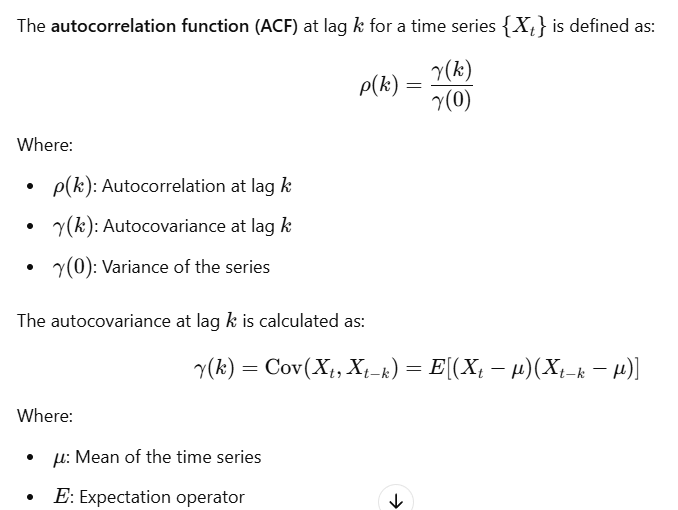
Calculating autocorrelation involves statistical formulas that measure the correlation between observations at different lags.

Mathematical Formula

• 

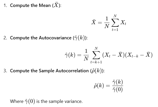
Sample Autocorrelation

In practice, we use the sample autocorrelation to estimate the true autocorrelation:

---

Terms Associated with Autocorrelation

Understanding autocorrelation involves several related terms and concepts.

Lag

• Definition: The number of time steps separating two observations in a time series.

• Notation:

  

Autocorrelation Function (ACF)

• Purpose: Describes how the autocorrelation coefficients vary with different lags.

• Usage: Helps identify the extent of correlation in a time series across various lags.

• Visualization: Often plotted as a correlogram (ACF plot).

Partial Autocorrelation Function (PACF)

• 

• Usage: Helps identify the appropriate number of autoregressive terms in ARIMA models.

• Visualization: Plotted as a PACF plot.

Stationarity

• Definition: A time series is stationary if its statistical properties (mean, variance, autocorrelation) are constant over time.

• Importance: Many time series models assume stationarity.

• Types:

  • Strong Stationarity: All moments are invariant over time.

  • Weak Stationarity: Mean and variance are constant; covariance depends only on lag.

White Noise

• Definition: A time series with a constant mean, constant variance, and zero autocorrelation at all lags.

• Implication: Indicates randomness; no predictable pattern exists.

---

Issues with Autocorrelation

Autocorrelation can lead to several problems, especially in regression analysis and statistical inference.

Impact on Statistical Inference

• Underestimated Standard Errors: Positive autocorrelation can cause standard errors to be underestimated.

• Type I Errors: Increased likelihood of incorrectly rejecting the null hypothesis.

Autocorrelation in Regression Residuals

• Definition: When residuals (errors) from a regression model are correlated with each other.

• Detection: Using tests like the Durbin-Watson statistic.

Violations of OLS Assumptions

Ordinary Least Squares (OLS) regression assumes that residuals are uncorrelated.

• Assumption Violation: Autocorrelation violates the independence assumption.

• Consequences:

  • OLS estimators remain unbiased but are inefficient.

  • Standard errors are biased, affecting hypothesis tests.

Spurious Regressions

• Definition: A regression that appears to have a significant relationship due to autocorrelation rather than a true underlying relationship.

• Cause: Non-stationary time series data can lead to misleading results.

Remedies for Autocorrelation

• Differencing: Transforming the series to reduce autocorrelation.

• Model Selection: Using models that account for autocorrelation (e.g., ARIMA).

• Newey-West Standard Errors: Adjusting standard errors to account for autocorrelation.

• Adding Lagged Variables: Including lagged dependent or independent variables.

---

Practical Implementation with Python

Let's explore how to calculate and interpret autocorrelation using Python libraries like pandas, numpy, matplotlib, and statsmodels.

Calculating and Plotting ACF and PACF

We can use the statsmodels library to compute and plot the ACF and PACF.

Example Code

Import Libraries

import numpy as np
import pandas as pd
import matplotlib.pyplot as plt

from statsmodels.tsa.stattools import acf, pacf
from statsmodels.graphics.tsaplots import plot_acf, plot_pacf

Generate Sample Time Series Data

# Create a synthetic time series with autocorrelation
np.random.seed(42)
n = 100
time = pd.date_range(start='2020-01-01', periods=n, freq='D')
data = np.zeros(n)

# Introduce autocorrelation
rho = 0.8  # Autocorrelation coefficient
e = np.random.normal(0, 1, n)
for t in range(1, n):
    data[t] = rho * data[t-1] + e[t]

df = pd.DataFrame({'Date': time, 'Value': data}).set_index('Date')

Plot the Time Series

plt.figure(figsize=(12, 6))
plt.plot(df['Value'], label='Time Series')
plt.title('Autocorrelated Time Series')
plt.xlabel('Date')
plt.ylabel('Value')
plt.legend()
plt.show()

Calculate ACF and PACF

# Calculate autocorrelation coefficients
lag_acf = acf(df['Value'], nlags=20)
lag_pacf = pacf(df['Value'], nlags=20, method='ols')

Plot ACF and PACF

# Plot ACF
plot_acf(df['Value'], lags=20)
plt.title('Autocorrelation Function (ACF)')
plt.show()

# Plot PACF
plot_pacf(df['Value'], lags=20)
plt.title('Partial Autocorrelation Function (PACF)')
plt.show()

Interpretation

• ACF Plot: Shows significant autocorrelation up to several lags, indicating that past values influence future values.

• PACF Plot: Helps determine the order of AR terms in ARIMA models.

---

Conclusion

Autocorrelation is a critical concept in time series analysis, reflecting the internal structure and dependencies within the data. Understanding autocorrelation allows analysts to:

• Identify Patterns: Detect whether current values depend on past values.

• Model Appropriately: Choose suitable models that account for autocorrelation (e.g., ARIMA).

• Avoid Misinterpretation: Recognize and mitigate issues like spurious regressions and violated assumptions.

Key Takeaways:

• Autocorrelation measures the relationship between a time series and its lagged values.

• Calculating autocorrelation involves statistical formulas for autocovariance and autocorrelation coefficients.

• Important terms include lag, ACF, PACF, stationarity, and white noise.

• Autocorrelation can lead to issues in statistical inference and regression analysis.

• Practical tools and methods exist to detect and address autocorrelation.

By incorporating the understanding of autocorrelation into time series analysis, you enhance the robustness and accuracy of your models and forecasts.

---