Understanding Exponential Smoothing: An In-Depth Guide

Exponential Smoothing is a family of forecasting methods that assign exponentially decreasing weights to past observations. These methods are widely used in time series forecasting due to their simplicity and effectiveness, especially when dealing with data that has trends and seasonality.

---

Table of Contents

1. Introduction to Exponential Smoothing

2. Simple Exponential Smoothing (SES)

   • Concept

   • Mathematical Formulation

   • Advantages and Disadvantages

   • Python Implementation

3. Double Exponential Smoothing (Holt's Method)

   • Concept

   • Mathematical Formulation

   • Advantages and Disadvantages

   • Python Implementation

4. Triple Exponential Smoothing (Holt-Winters Method)

   • Concept

   • Mathematical Formulation

   • Advantages and Disadvantages

   • Python Implementation

5. Conclusion

6. References

---

Introduction to Exponential Smoothing

Exponential Smoothing methods are a set of time series forecasting techniques that apply decreasing weights to past observations. The weights decrease exponentially as the observations get older, hence the name "exponential smoothing."

Key Characteristics

• Weighted Averages: Recent observations have more influence on the forecast than older ones.

• Adaptability: Can be adapted to capture trends and seasonal patterns.

• Simplicity: Easy to implement and computationally efficient.

---

Simple Exponential Smoothing (SES)

Concept

Simple Exponential Smoothing is suitable for forecasting time series data that does not exhibit any systematic trends or seasonal patterns. It forecasts future values based solely on past observations, with more weight given to recent observations.

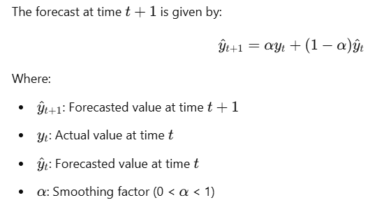
Mathematical Formulation

Advantages and Disadvantages

Advantages:

• Simplicity: Easy to understand and implement.

• Requires Minimal Data: Only past observations are needed.

• Good for Stationary Data: Effective when data lacks trends and seasonality.

Disadvantages:

• Cannot Handle Trends: Ineffective for data with upward or downward trends.

• Not Suitable for Seasonality: Cannot model seasonal patterns.

• 

Python Implementation

Import Libraries

import numpy as np
import pandas as pd
import matplotlib.pyplot as plt
from statsmodels.tsa.holtwinters import SimpleExpSmoothing

Create Sample Data

# Generate synthetic stationary data
np.random.seed(42)
data = np.random.normal(loc=50, scale=5, size=100)
index = pd.date_range(start='2020-01-01', periods=100, freq='D')
df = pd.DataFrame(data, index=index, columns=['Value'])

Apply Simple Exponential Smoothing

# Initialize and fit the model
model = SimpleExpSmoothing(df['Value'])
model_fit = model.fit(smoothing_level=0.2, optimized=False)

# Forecast
df['SES_Forecast'] = model_fit.fittedvalues

Visualize the Results

plt.figure(figsize=(12, 6))
plt.plot(df['Value'], label='Actual')
plt.plot(df['SES_Forecast'], label='SES Forecast', color='red')
plt.title('Simple Exponential Smoothing')
plt.xlabel('Date')
plt.ylabel('Value')
plt.legend()
plt.show()

---

Double Exponential Smoothing (Holt's Method)

Concept

Double Exponential Smoothing, also known as Holt's Method, extends SES by introducing a component to model the trend in the data. It is suitable for time series data with a linear trend but without seasonality.

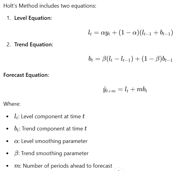
Mathematical Formulation

Advantages and Disadvantages

Advantages:

• Captures Trends: Effective for data with linear trends.

• Simple Extension of SES: Builds upon the simplicity of SES.

Disadvantages:

• Not Suitable for Seasonality: Cannot handle seasonal fluctuations.

  

Python Implementation

Create Sample Data with Trend

# Generate synthetic data with a trend
np.random.seed(42)
trend = np.arange(100) * 0.5
noise = np.random.normal(loc=0, scale=2, size=100)
data = 50 + trend + noise
index = pd.date_range(start='2020-01-01', periods=100, freq='D')
df = pd.DataFrame(data, index=index, columns=['Value'])

Apply Holt's Method

from statsmodels.tsa.holtwinters import ExponentialSmoothing

# Initialize and fit the model
model = ExponentialSmoothing(df['Value'], trend='add', seasonal=None)
model_fit = model.fit(smoothing_level=0.8, smoothing_slope=0.2, optimized=False)

# Forecast
df['Holt_Forecast'] = model_fit.fittedvalues

Visualize the Results

plt.figure(figsize=(12, 6))
plt.plot(df['Value'], label='Actual')
plt.plot(df['Holt_Forecast'], label='Holt\'s Forecast', color='red')
plt.title('Double Exponential Smoothing (Holt\'s Method)')
plt.xlabel('Date')
plt.ylabel('Value')
plt.legend()
plt.show()

---

Triple Exponential Smoothing (Holt-Winters Method)

Concept

Triple Exponential Smoothing, known as the Holt-Winters Method, extends Holt's Method by adding a seasonal component. It is suitable for time series data with trends and seasonal patterns.

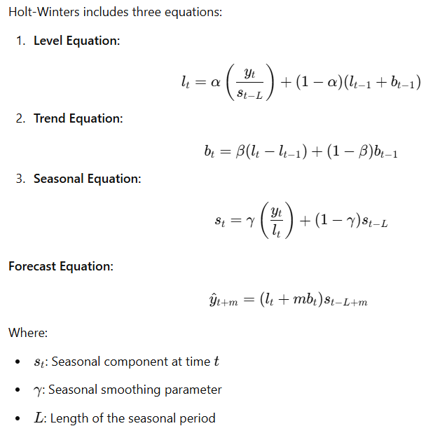
Mathematical Formulation

Advantages and Disadvantages

Advantages:

• Models Seasonality: Effective for data with seasonal patterns.

• Flexible: Can handle both additive and multiplicative seasonality.

Disadvantages:

• Complexity: More complex due to additional parameters.

• Risk of Overfitting: Requires careful parameter tuning to avoid overfitting.

Python Implementation

Create Sample Data with Trend and Seasonality

# Generate synthetic data with trend and seasonality
np.random.seed(42)
periods = 200
seasonal_periods = 12
trend = np.arange(periods) * 0.2
seasonality = 10 + 5 * np.sin(2 * np.pi * np.arange(periods) / seasonal_periods)
noise = np.random.normal(loc=0, scale=2, size=periods)
data = 50 + trend + seasonality + noise
index = pd.date_range(start='2020-01-01', periods=periods, freq='M')
df = pd.DataFrame(data, index=index, columns=['Value'])

Apply Holt-Winters Method

# Initialize and fit the model
model = ExponentialSmoothing(
    df['Value'],
    trend='add',
    seasonal='add',
    seasonal_periods=seasonal_periods
)
model_fit = model.fit()

# Forecast
df['HW_Forecast'] = model_fit.fittedvalues

Visualize the Results

plt.figure(figsize=(12, 6))
plt.plot(df['Value'], label='Actual')
plt.plot(df['HW_Forecast'], label='Holt-Winters Forecast', color='red')
plt.title('Triple Exponential Smoothing (Holt-Winters Method)')
plt.xlabel('Date')
plt.ylabel('Value')
plt.legend()
plt.show()

Forecasting Future Values

# Forecast the next 24 periods
forecast_periods = 24
forecast = model_fit.forecast(forecast_periods)

# Create forecast index
forecast_index = pd.date_range(
    start=df.index[-1] + pd.DateOffset(months=1),
    periods=forecast_periods,
    freq='M'
)

# Plot the forecast
plt.figure(figsize=(12, 6))
plt.plot(df['Value'], label='Actual')
plt.plot(df['HW_Forecast'], label='Fitted', color='red')
plt.plot(forecast_index, forecast, label='Forecast', color='green')
plt.title('Holt-Winters Method Forecast')
plt.xlabel('Date')
plt.ylabel('Value')
plt.legend()
plt.show()

---

Conclusion

Exponential Smoothing methods provide a versatile set of tools for time series forecasting, adaptable to various data characteristics.

Summary of Methods

1. Simple Exponential Smoothing (SES):

   • Use Case: Data without trend or seasonality.

   • Advantage: Simplicity.

   • Disadvantage: Cannot model trends or seasonality.

2. Double Exponential Smoothing (Holt's Method):

   • Use Case: Data with a linear trend but no seasonality.

   • Advantage: Captures trends.

   • Disadvantage: Cannot model seasonal patterns.

3. Triple Exponential Smoothing (Holt-Winters Method):

   • Use Case: Data with trend and seasonality.

   • Advantage: Models both trend and seasonal components.

   • Disadvantage: Increased complexity and risk of overfitting.

Advantages of Exponential Smoothing

• Flexibility: Can be tailored to different types of time series data.

• Efficiency: Computationally efficient, suitable for real-time forecasting.

• Adaptability: Parameters can be optimized for better forecasting performance.

Disadvantages of Exponential Smoothing

• Parameter Sensitivity: Forecast accuracy depends on the choice of smoothing parameters.

• Assumption of Linearity: May not perform well with non-linear patterns.

• Limited to Univariate Series: Does not consider external variables or covariates.

---

References

• Hyndman, R. J., & Athanasopoulos, G. (2018). Forecasting: Principles and Practice. OTexts. Online Version

• Statsmodels Documentation: Exponential Smoothing

• Brown, R. G. (1959). Statistical Forecasting for Inventory Control. McGraw Hill.

---