Quick Guide to a Unified Batch-Stream Computing Platform
 DolphinDB
1. Overview
This tutorial describes how to build a DolphinDB-based computing platform that supports both batch and stream processing with high extensibility and compatibility. The platform allows for the calculation of minute-level factors from high-frequency data, as well as more complex factors derived from these.
Quant researchers can input factor expressions through the platform interface and obtain the results without needing to understand the underlying streaming architecture.
With the computing platform, the same factor expression can be used in development and production environments without rewriting. This reduces costs and boosts efficiency across the entire development-to-production workflow.
2. Unified Batch-Stream Computing Platform for Level 2 Market Data
2.1 Usage and Deployment Workflows
The image below shows how quant researchers can leverage historical data for factor development using the computing platform:

In the DolphinDB IDE (the “GUI”), quant researchers develop factors by coding expressions and functions in scripts. These scripts are executed through the computing platform interface to obtain results. Syntax errors will generate an error message.
Once factors are validated, deployment to production for real-time computing is required. The image below shows the deployment process:
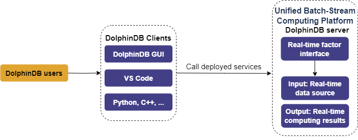
After deployment, table objects representing the input and output of the computing service are automatically created. Input tables receive real-time data streamed through tools provided by DolphinDB, while output tables store the computed results.
2.2 Platform Architecture
The architecture of the computing platform is shown below:
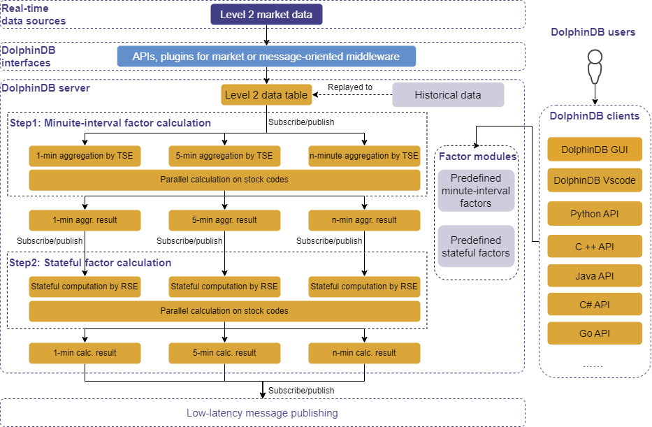
Note: In the diagram, the time-series engine is abbreviated as “TSE” and the reactive state engine as “RSE” for brevity.
The platform provides the following features:
Real-time data ingestionthrough:
various APIs (C++, Java, etc.)
market data plugins
plugins for message-oriented middleware (Kafka, zmq, MQTT, etc.)
Data replay of one or multiple datasets at controlled speeds while preserving timestamp order. This enables backtesting factors by replaying historical data as live streams.
Built-in streaming engines for time-series analysis: In this tutorial, the time-series engine calculates factors at minute intervals by applying tumbling window aggregation to high frequency data. Further, the reactive state engine consumes these minute-factors as inputs to derive more complex factors.
Integrated development environment (IDE): Quant researchers can use the DolphinDB GUI and the DolphinDB plugin for Visual Studio Code as IDEs for factor development and testing. Additionally, researchers can also interact with the server through DolphinDB APIs to get the real-time results from the computing service.
Low-latency message publishing: DolphinDB provides plugins for publishing real-time calculation results to message queues like Kafka, zmq, RabbitMQ, and MQTT.
2.3 Computing Capabilities
The computing platform demonstrated in this tutorial computes two kinds of factors based on level 2 market data:
(1) Minute-interval factors
Minute-interval factors are calculated by applying aggregations using fixed-size tumbling windows on high-frequency market data, such as computing OHLC bars at one-minute or multi-minute intervals. These factors are calculated using the time-series engine (createTimeSeriesEngine).
(2) Stateful factors
In this tutorial, the stateful factors (e.g., EMA and RSI) are derived fromminute-interval factors. The reactive state engine (createReactiveStateEngine) handles these factors by applying sliding windows on high-frequency market data. The windows slide row-by-row, with the window size determined either by a fixed row count or a specified time range.
2.4 Defining Factors
2.4.1 Defining Minute-Interval Factors
The time-series engine calculates minute-interval factors. It has optimized the following built-in aggregate functions to enable incremental computing: corr, covar, first, last, max, med, min, percentile, quantile, std, var, sum, sum2, sum3, sum4, wavg, wsum, count, firstNot, ifirstNot, lastNot, ilastNot, imax, imin, nunique, prod, sem, mode, searchK, beta, avg. Factors constructed directly from these functions can thus be computed incrementally. For minute-interval factors not defined solely by these optimized functions, users must specify them with the defgstatement.
The following examples explain the differences in factor definition.
- Defining Incrementally Computed Factors
def High(){
    return "max(LastPx)"
}
The High factor indicates the highest price over a specified time interval by returning the maximum value in each window. It leverages the max()aggregate function by passing it the latest trade price (lastPx). The platform parses the "max(LastPx)" string as metacode <max(LastPx)> and passes it to the time-series engine.
Similarly, calculating the open, close and low prices at specified intervals can be achieved using the optimized first(), last(), and min() functions:
def Open(){
 return "first(LastPx)"
}
def Close(){
 return "last(LastPx)"
}
def Low(){
 return "min(LastPx)"
}
- Defining Factors Not Incrementally Computed
defg Press(BidPrice0,BidPrice1,BidPrice2,BidPrice3,BidPrice4,BidPrice5,BidPrice6,BidPrice7,BidPrice8,BidPrice9,BidOrderQty0,BidOrderQty1,BidOrderQty2,BidOrderQty3,BidOrderQty4,BidOrderQty5,BidOrderQty6,BidOrderQty7,BidOrderQty8,BidOrderQty9,OfferPrice0,OfferPrice1,OfferPrice2,OfferPrice3,OfferPrice4,OfferPrice5,OfferPrice6,OfferPrice7,OfferPrice8,OfferPrice9,OfferOrderQty0,OfferOrderQty1,OfferOrderQty2,OfferOrderQty3,OfferOrderQty4,OfferOrderQty5,OfferOrderQty6,OfferOrderQty7,OfferOrderQty8,OfferOrderQty9){
 bidPrice = matrix(BidPrice0,BidPrice1,BidPrice2,BidPrice3,BidPrice4,BidPrice5,BidPrice6,BidPrice7,BidPrice8,BidPrice9)
 bidQty = matrix(BidOrderQty0,BidOrderQty1,BidOrderQty2,BidOrderQty3,BidOrderQty4,BidOrderQty5,BidOrderQty6,BidOrderQty7,BidOrderQty8,BidOrderQty9)
 offerPrice = matrix(OfferPrice0,OfferPrice1,OfferPrice2,OfferPrice3,OfferPrice4,OfferPrice5,OfferPrice6,OfferPrice7,OfferPrice8,OfferPrice9)
 offerQty = matrix(OfferOrderQty0,OfferOrderQty1,OfferOrderQty2,OfferOrderQty3,OfferOrderQty4,OfferOrderQty5,OfferOrderQty6,OfferOrderQty7,OfferOrderQty8,OfferOrderQty9)
 wap = (bidPrice[0]*offerQty[0] + offerPrice[0]*bidQty[0])\(bidQty[0]+offerQty[0])
 bidw=(1.0\(bidPrice-wap))
 bidw=bidw\(bidw.rowSum())
 offerw=(1.0\(offerPrice-wap))
 offerw=offerw\(offerw.rowSum())
 press = log((bidQty*bidw).rowSum())-log((offerQty*offerw).rowSum())
 return avg(press)
}
The Press factor measures the price pressure in the market. BidPrice, BidOrderQty, OfferPrice and OfferOrderQty are the 10 best bid/offer prices and volumes. The following expressions explain how the factor is implemented:
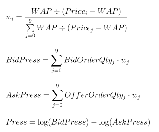
The factor is too complex to be calculated using only the built-in optimized aggregate functions. It requires a user-defined aggregate function defined with the defg statement. The computing platform automatically converts the Press function to the metacode <Press()> and passes it to the time-series engine.
2.4.2 Defining Stateful Factors
The reactive state engine calculates factors dependent on historical state. For such stateful factors, performing full recomputation on each update is inefficient. Optimizing for incremental calculation in stream computing is thus critical. The following state functions have been optimized in the reactive state engine to enable efficient incremental computing:
cumulative function: cumavg, cumsum, cumprod, cumcount, cummin, cummax, cumvar, cumvarp, cumstd, cumstdp, cumcorr, cumcovar, cumbeta, cumwsum, cumwavg, cumfirstNot, cumlastNot, cummed, cumpercentile, cumnunique, cumPositiveStreak, cummdd
moving function: ema, mavg, msum, mcount, mprod, mvar, mvarp, mstd, mstdp, mskew, mkurtosis, mmin, mmax, mimin, mimax, mmed, mpercentile, mrank, mcorr, mcovar, mbeta, mwsum, mwavg, mmad, mfirst, mlast, mslr, tmove, tmfirst, tmlast, tmsum, tmavg, tmcount, tmvar, tmvarp, tmstd, tmstdp, tmprod, tmskew, tmkurtosis, tmmin, tmmax, tmmed, tmpercentile, tmrank, tmcovar, tmbeta, tmcorr, tmwavg, tmwsum, tmoving, moving, sma, wma, dema, tema, trima, linearTimeTrend, talib, t3, ma, mmaxPositiveStreak
order-sensitive function: deltas, ratios, ffill, move, prev, iterate, ewmMean, ewmVar, ewmStd, ewmCov, ewmCorr, prevState, percentChange
For more optimized state functions, see createReactiveStateEngine.
The following script defines the MACD factor:
@state
def MACD(Close, SHORT_ = 12, LONG_ = 26, M = 9) {
    DIF = ewmMean(Close, span = SHORT_, adjust = false) - ewmMean(Close, span = LONG_, adjust = false)
    DEA = ewmMean(DIF, span = M, adjust = false)
    MACD = (DIF - DEA) * 2
    return round(DIF, 3), round(DEA, 3), round(MACD, 3)
}
Note: When defining a stateful function (i.e., the current result depends on results calculated so far), add @state before the function definition.
The MACD factor takes Close (closing price aggregated at minute intervals) as an input parameter. Close must be included in the output of the time-series engine.
3. Service Deployment and Factor Development
3.1 Deploying the Computing Service
Step 1.
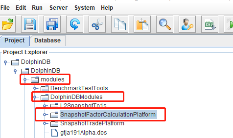
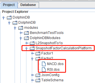
Import the modules of the computing platform (see appendix SnapshotFactorCalculationPlatform) to the DolphinDB GUI. The directory must be the same as shown in the image below:
Step 2.
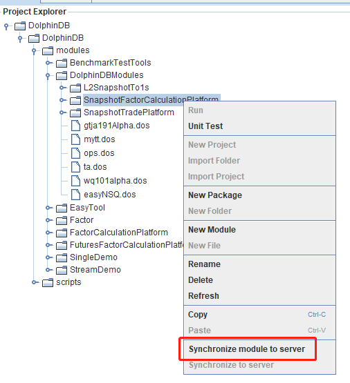
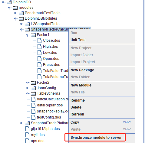
Right-click SnapshotFactorCalculationPlatform, and select Synchronize module to server from the menu.
Step 3.
To check whether the platform has been successfully deployed to the DolphinDB server, create a script under the scripts directory with the following code:
use DolphinDBModules::SnapshotFactorCalculationPlatform::JsonConfig::JsonConfigLoad

/**
The service deployment function takes the following arguments:
testConfig.dos: an example configuration file in JSON format
parallel: specifies the level of parallelism in computation
 */
jsonPath = "./modules/DolphinDBModules/SnapshotFactorCalculationPlatform/testConfig.dos"
parallel = 2
//call the service deployment function
loadJsonConfig(jsonPath, parallel)
Once the script is successfully executed, tables representing the input and outputs of the computing service are displayed in the GUI’s Variables view.
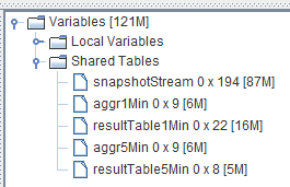
Users simply need to ingest real-time data or historical data into the service input table (the “snapshotStream” table), and the results can be found in the output tables.
3.2 Developing Factors
Step 1. Defining Factor Expressions
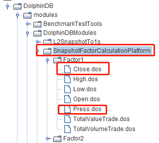
Scripts for minute-interval factors are saved under DolphinDB GUI > SnapshotFactorCalculationPlatform > Factor1. Once the computing platform is deployed (see section 3.1), we can find several predefined minute-interval factors, as shown in the image below. (In this example, the scripts for Close and Press are used for demonstration.)
Scripts for stateful factors are saved under DolphinDB GUI > SnapshotFactorCalculationPlatform > Factor2. The computing platform provides several predefined stateful factors under the directory, as shown in the image below. (In this example, the scripts for MACD and RSI are used for demonstration.)
Once users finished defining new factors, they need to synchronize the scripts to the DolphinDB server.
Step 2. Generate Configuration File
Create a script under DolphinDB GUI > scripts with the following code to generate a JSON configuration file:
use DolphinDBModules::SnapshotFactorCalculationPlatform::JsonConfig::JsonGetFileString

//specify the configuration parameters for minute-interval factors
FactorLevel1 = `Close`Press`Close`Press
isInc = `true`false`true`false
barMinutesLevel1 = 1 1 5 5
useSystemTime = `false`false`false`false

//specify the configuration parameters for stateful factors
FactorLevel2 = `RSI`MACD`RSI`MACD
barMinutesLevel2 = [[1, 1], [1], [5], [5]]
colNameLevel2 = [`RSI, `DIF`DEA`MACD, `RSI, `DIF`DEA`MACD]
paramsName = [`N, `SHORT_`LONG_`M, `N,`SHORT_`LONG_`M]
paramsValue = [[[24], [30]], [[18, 30, 10]], [[24]], [[9, 25, 6]], [[12, 26, 9]]]

// specify the path to save the JSON file
jsonPath = "./test.json"
JsonFileString = JsonGetFileString(FactorLevel1, isInc, barMinutesLevel1, useSystemTime, FactorLevel2, barMinutesLevel2, colNameLevel2, paramsName, paramsValue)
saveTextFile(JsonFileString, jsonPath)
Configuration parameters for minute-level factors:
FactorLevel1 specifies the names of the minute-interval factors, e.g Close and Press. These factors should already be defined and synchronized to the DolphinDB server as described in step 1.
isInc has the same length as FactorLevel1, indicating whether the specified factors implement incremental computing.
barMinutesLevel has the same length as FactorLevel1, indicating the frequency (in unit of minutes) at which the factors are computed.
useSystemTime has the same length as FactorLevel1, indicating how window calculations are triggered. True means each calculation is triggered based on the system time, and false means it is triggered by event time. Factors calculated at the same intervals must adopt the same triggering method.
Configuration parameters for stateful factors:
FactorLevel2 specifies the names of the stateful factors, e.g., RSI and MACD. These factors should already be defined and synchronized to the DolphinDB server as described in step 1.
barMinutesLevel2 has the same length as FactorLevel2, indicating the number of times a factor will be calculated and the window size that applies to each calculation.For example, the first element [1,1] means to perform two separate calculations of
FactorLevel2[0](i.e., the RSI factor) at 1-minute intervals. The window size for each calculation is specified by paramsValue.colNameLevel2 has the same length as FactorLevel2, indicating the output column names corresponding to each calculated factor value.
paramsName has the same length as FactorLevel2, indicating the parameters for each factor.
paramsValue has the same length as FactorLevel2, and each element corresponds to an element of barMinutesLevel2. For example, the first element of paramsValue is [[24], [30]], which aligns with
barMinutesLevel2[0](i.e., [1, 1]). This indicates that window calculations will be performed twice onFactorLevel2[0](the RSI factor) for every minute, with window sizes of 24 and 30, respectively.
Once the script is executed, a configuration file test.json is generated under the DolphinDB server directory with the following contents:
[{"factor": "Close", "isInc": true, "barMinute": 1, "level": 1, "useSystemTime": false}, {"factor": "Press", "isInc": false, "barMinute": 1, "level": 1, "useSystemTime": false}, {"factor": "Close", "isInc": true, "barMinute": 5, "level": 1, "useSystemTime": false}, {"factor": "Press", "isInc": false, "barMinute": 5, "level": 1, "useSystemTime": false}, {"factor": "RSI", "level": 2, "colName": `R_1, "barMinute": 1, "N": 24}, {"factor": "RSI", "level": 2, "colName": `R_2, "barMinute": 1, "N": 30}, {"factor": "MACD", "level": 2, "colName": `DIF_1`DEA_1`MACD_1, "barMinute": 1, "SHORT_": 18, "LONG_": 30, "M": 10}, {"factor": "RSI", "level": 2, "colName": `R_1, "barMinute": 5, "N": 24}, {"factor": "MACD", "level": 2, "colName": `DIF_1`DEA_1`MACD_1, "barMinute": 5, "SHORT_": 9, "LONG_": 25, "M": 6}]
Step 3. Deploy Computing Service
To deploy the computing service, create a script under DolphinDB GUI > scripts and execute the following code:
//call the service deployment function
use DolphinDBModules::SnapshotFactorCalculationPlatform::JsonConfig::JsonConfigLoad
jsonPath = "./test.json"
parallel = 1
loadJsonConfig(jsonPath, parallel)
Note: Before executing the script above, clear up the environment.
Step 4. Calculate the factors
Save the CSV file containing test data (see appendix test_scripts.zip) to the DolphinDB server. In this example, the CSV file is saved at /hdd/hdd9/tutorials/SnapshotFactorCalculationPlatform/test.csv.
To ingest the test data into the computing platform as a stream through replay, create a script with the following code under DolphinDB GUI > scripts:
use DolphinDBModules::SnapshotFactorCalculationPlatform::snapshotReplay
csvPath = "/hdd/hdd9/tutorials/SnapshotFactorCalculationPlatform/test.csv"
snapshotCsvReplayJob(csvPath, snapshotStream)
Refresh the DolphinDB GUI. The result tables in the Variables view are updated at each execution. The screenshot below shows the result table for the 1-minute interval factors:
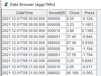
The screenshot below shows the result table for the stateful factors calculated at 1-minute intervals:

The “CostTime” column indicates the microseconds elapsed for each calculation.
3.3 Deploying the Computing Service from Python and Subscribing to Results
Procedures described in this section are performed in the Jupyter notebook.
Version details:
DolphinDB server 2.00.9.2
DolphinDB Python API 1.30.21.1
Python 3.7.6
Step 1.
Import the dolphindb package and the dependent library. Then connect to the DolphinDB server.
import dolphindb as ddb
import numpy as np

s = ddb.session(host="localhost", port=8892, userid='admin', password='123456',enablePickle=False)
Step 2.
Prerequisite:
The JSON configuration file has been generated on the server. For details, see “step 2. Generate Configuration File” in section 3.2 Developing Factors.
Initialize the environment in the DolphinDB server.
Deploy the computing service:
jsonPath = "./modules/DolphinDBModules/SnapshotFactorCalculationPlatform/testConfig.dos"
parallel = 1
scripts = """
    use DolphinDBModules::SnapshotFactorCalculationPlatform::JsonConfig::JsonConfigLoad
    loadJsonConfig("{0}", {1})
""".format(jsonPath, parallel)
s.run(scripts)
jsonPath specifies the relative path to the default configuration file on the DolphinDB server.
Step 3.
Replay historical data:
csvPath = "/hdd/hdd9/tutorials/SnapshotFactorCalculationPlatform/test.csv"
scripts = """
    use DolphinDBModules::SnapshotFactorCalculationPlatform::snapshotReplay
    snapshotCsvReplayJob("{0}", snapshotStream)
""".format(csvPath)
s.run(scripts)
csvPath specifies the absolute path to the test data CSV file (see Appendix) on the DolphinDB server machine. In this example, the test data is saved at /hdd/hdd9/tutorials/SnapshotFactorCalculationPlatform/test.csv.
Step 4.
Submit a query and download the result to Python:
queryDate = "2021.12.01"
SecurityID = "600000"
scripts = """
    select * from resultTable1Min where date(DateTime)={0}, SecurityID="{1}"
""".format(queryDate, SecurityID)
resultdf = s.run(scripts)
resultdf
Sample data of resultdf:

Step 5.
On the Python client, subscribe to the result table on the DolphinDB server:
s.enableStreaming(0)
def handler(lst):
    print(lst)
s.subscribe(host="localhost", port=8892, handler=handler, tableName="aggr1Min", actionName="sub1min", offset=0, msgAsTable=False,  filter=np.array(['600010']))
The offset parameter of s.ubscribe is set to 0, indicating the subscription starts from the first row of the result table:

To cancel subscription, execute the following script:
s.unsubscribe(host="localhost", port=8892,tableName="aggr1Min",actionName="sub1min")
After you have finished, it is recommended to manually close the current session in Python:
s.close()
For C++, Java and other languages, the server-client communication works similarly to Python. Refer to the official API documentation for details.
3.4 Pushing Real-Time Results to Kafka
Results of computations performed by the DolphinDB server can be pushed in real-time to a low-latency message bus on the local machine. To illustrate this process, in the following example, we push the results of 1-minute factors to Kafka.
Prerequisites: (1) A topic for aggr1Min has been created in Kafka. (2) The Kafka plugin has been loaded in DolphinDB.
To push the results to Kafka, create a script under DolphinDB GUI > scripts with the following code:
use DolphinDBModules::SnapshotFactorCalculationPlatform::resultToKafka

producer = initKafkaProducer("localhost:9092")
subscribeTable(tableName="aggr1Min", actionName="aggr1MinToKafka", offset=0, handler=aggr1MinToKafka{producer, "aggr1Min"}, msgAsTable=true)
initKafkaProducer("localhost:9092") specifies the IP address and port number of the Kafka service.
The calculation results can be consumed from Kafka:

The DolphinDB monitoring log shows that it takes about 180 microseconds on average to push results from DolphinDB to Kafka:

4. FAQs
4.1 Minute-Interval Factors Calculated by the Time-Series Engine
- Should calculation windows be triggered by system time or events?
The computing platform demonstrated in this tutorial defaults to using events to trigger window calculations. However, DolphinDB’s time-series engine allows configuration of the useSystemTime parameter to change this setting.
- If windows are triggered by events, how do you ensure that windows calculating inactive stocks are triggered at some point?
The computing platform demonstrated in this tutorial groups data by individual stocks, and there is no built-in force triggering mechanism across these groups. Nonetheless, DolphinDB’s time-series engine provides the forceTriggerTime parameter, offering a solution to trigger inactive windows.
- If windows are triggered by events, how to make sure the windows at lunch breaks, or at the end of a continuous auction session, are triggered?
The computing platform demonstrated in this tutorial does not cover such scenarios. However, DolphinDB’s daily time-series engine provides the forceTriggerSessionEndTime parameter, which can be configured to meet specific requirements.
- Is the left boundary of the calculation windows inclusive or exclusive?
The computing platform demonstrated in this tutorial uses window with an inclusive left boundary and an exclusive right boundary. DolphinDB’s time-series engine provides the closed parameter, allowing you to modify this setting.
- Does the time column in the result indicate the start time of each window, or the end time?
The computing platform demonstrated in this tutorial uses the window start time. DolphinDB’s time-series engine provides the useWindowStartTime parameter, providing flexibility to modify this setting.
- If a window doesn’t include any data from a certain group, can I fill the result of that window with the previous window’s result or a specified value?
The computing platform demonstrated in this tutorial does not adopt any filling rules. However, DolphinDB’s time-series engine provides the fillparameter. You can use fill to specify the filling method when a window does not contain any data from a group. Options include “none” (outputting nothing), “null” (outputting a NULL value), “ffill” (outputting the result of the previous window), or specifying a specific value as the output, which must be of the same type as the corresponding factor.
4.2 Stateful Factors Calculated by the Reactive State Engine
- Suppose I have 1,000 factors that all use a common intermediate variable. How can I prevent repeated calculations?
Define a separate function to calculate the intermediate variable. For example, factor1 and factor2 are two factors to be calculated in the computing platform demonstrated in this tutorial. The definitions are as follows:
@state
def factor1(price) {
    a = ema(price, 20)
    b = ema(price, 40)
    tmp = 1000 * (a-b)\(a+b)
    return  ema(tmp , 10) - ema(tmp , 20)
}
@state
def factor2(price) {
    a = ema(price, 20)
    b = ema(price, 40)
    tmp = 1000 * (a-b)\(a+b)
    return  mavg(tmp, 10)
}
As shown in the scripts, both factor1 and factor2 depend on the tmp variable. To avoid repeated calculation of tmp, define a function tmpFactor:
@state
def tmpFactor(price) {
    a = ema(price, 20)
    b = ema(price, 40)
    tmp = 1000 * (a-b)\(a+b)
    return  tmp
}
Then rewrite the definitions of factor1 and factor2 as follows:
@state
def factor1(price) {
    tmp = tmpFactor(price)
    return  ema(tmp , 10) - ema(tmp , 20)
}
@state
def factor2(price) {
    tmp = tmpFactor(price)
    return  mavg(tmp, 10)
}
By doing so, DolphinDB’s reactive state engine will automatically avoid repeated calculations of the same variable when parsing stateful factors.
Appendix
Subscribe to my newsletter
Read articles from DolphinDB directly inside your inbox. Subscribe to the newsletter, and don't miss out.
Written by
