Fundamentals of Generative Models

Introduction to Generative Models

Generative Machine Learning is a subset of artificial intelligence, where models are trained to generate new data samples like the original training data. Generative machine learning involves the development of models that learn the underlying distribution of the training data. These models can generate new data samples, which have similar characteristics to the original dataset. Fundamentally, generative models aim to understand the core of the data to generate unique and diverse outputs. Generative models must learn the entire data distribution instead of just learning the decision boundary like discriminative models.

A generative model is a model of the conditional probability of the observable ‘X’ , given the condition ‘Y’ and a target ‘y’ , symbolically can be represented as

Bayesian networks: Bayesian Network (Bayes Network) is a probabilistic graphical model that represents a set of variables and their conditional dependencies via a directed acyclic graph (DAG). These networks are used to model uncertainty and to infer the likelihood of outcomes based on known evidence. Each node in the graph represents a random variable, which can be discrete or continuous. While the edges indicate direct dependencies between the variables. A directed edge from node A to node B implies that B is conditionally dependent on A. This can be represented by probability distribution

Because a Bayesian network is a complete model for its variables and their relationships, it can be used to answer probabilistic queries about the variables. For example, the network can be used to update information pertaining to a subset of variables when other variables are observed. This process of computing the posterior distribution of variables given evidence is called probabilistic inference.

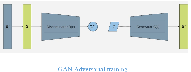
Generative Adversarial Networks (GANs): Generative Adversarial Networks (GANs) A generative adversarial network (GAN) is a deep learning architecture which trains two neural networks to compete against each other to generate more authentic new data from a given training dataset. The two neural networks are known as generator and discriminator, which work against each other in a game-like setup. The generator network tries to produce fake data that resembles real data. It starts with random noise and generates samples that get progressively closer to the real distribution over time. The discriminator network is like a classifier. It takes input (either real or generated) and tries to determine whether the sample is real or fake. Its goal of generator network is to "trick" the discriminator by producing data indistinguishable from the real data.

Initially, the generator creates random data that can be easily identified as fake. But as it learns, it improves. The discriminator learns to identify the fake samples while improving its ability to recognize real data.

The two networks are trained simultaneously in a zero-sum game: the generator tries to minimize the discriminator’s ability to distinguish between real and fake, while the discriminator tries to maximize its ability to correctly classify. This adversarial process pushes the generator to create increasingly realistic samples. Over time, the generator can produce data that is nearly indistinguishable from the real data.

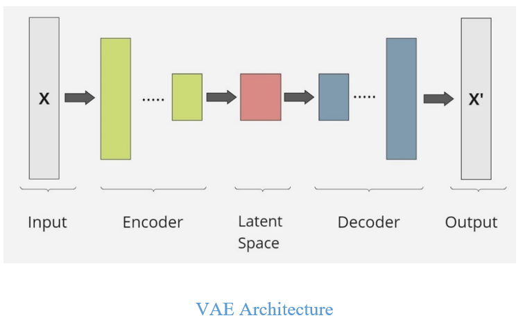
Variational Autoencoders (VAEs): Variational Autoencoders (VAEs) are type of autoencoders used to generate new data points that are similar to a given dataset. Like standard autoencoders, VAEs consist of an 'encoder' and a 'decoder' network. VAEs combines concepts from autoencoders and probabilistic graphical models, using variational Bayesian methods to generate new data by mapping inputs (like images) into a probabilistic latent space, often modeled as a multivariate Gaussian distribution. The encoder transforms data into this distribution, while the decoder reconstructs data from it. This probabilistic mapping helps avoid overfitting.

The encoder takes an input and maps it to a latent space. However, unlike standard autoencoders that map to a fixed latent vector, VAEs map to a probability distribution over the latent space, usually a Gaussian distribution. This allows the model to learn uncertainty in the data. Instead of sampling directly from the distribution, VAEs use a technique called the reparameterization trick or stochastic backpropagation. This trick allows gradients to flow through the stochastic sampling process, which is critical for training via backpropagation. The key idea is to express the sampling from a distribution as a deterministic function with an added random variable. The decoder maps the latent representation (sampled from the distribution) back into the original data space, aiming to reconstruct the original input. The decoder tries to generate a new data point from the sampled latent vector, which should resemble real data.

The loss function in a VAE consists of two parts: Reconstruction Loss and Regularization Loss. Reconstruction Loss is the error between the original input and the reconstruction produced by the decoder. While Regularization Loss measures how much the learned distribution (the output of the encoder) deviates from the prior distribution (typically a standard Gaussian). The goal is to make the learned distribution as close as possible to a standard normal distribution while still accurately representing the data.

Unlike GANs, VAEs are typically easier to train and come with probabilistic guarantees, but the samples they generate may not be as sharp or realistic as those from GANs. VAEs offer an interpretable latent space, making them useful for tasks where understanding the latent structure is important.

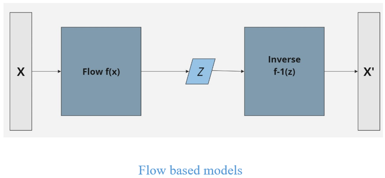
Flow-based models: - Flow-based models are probabilistic generative models that define a complex probability distribution by transforming a simple one (like a Gaussian distribution) by leveraging normalizing flow. These models aim to learn the transformation between a simple, known distribution and the target distribution of the data, enabling both density estimation and sample generation.

Each transformation function in a flow-based model must be invertible, meaning that you can map data from the simple distribution and back. This property is crucial for both training and generation. Flow-based models leverage the change of variables formula from probability theory to compute the probability density of data points. If ‘f’ is an invertible transformation and ‘x’ is a data point, then the probability of ‘x’ under the model is computed as:

The model is typically trained by maximizing the log-likelihood of the data. Since the transformations are invertible, the log-likelihood can be directly computed, making flow-based models advantageous for tasks like density estimation. Once trained, flow-based models can generate new data by sampling from the simple distribution and applying the inverse of the learned transformations to get new samples from the target distribution. Flow-based models can estimate the likelihood of data points, making them useful for anomaly detection as well, where unusual points have low probability densities.

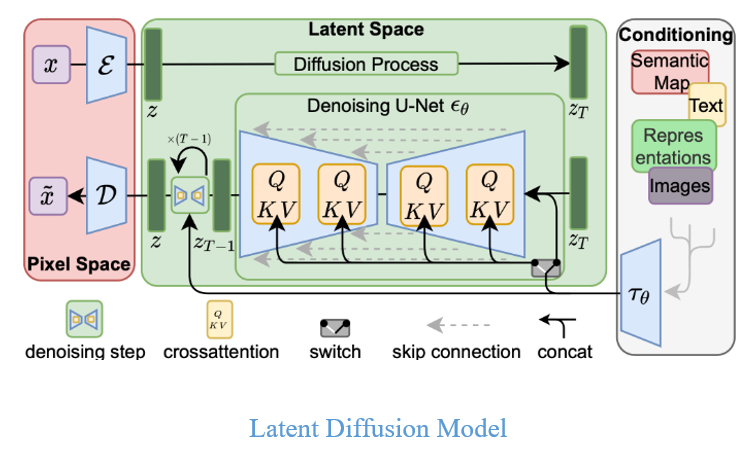
Diffusion models: Diffusion models produce data, such as images, by gradually transforming simple noise into structured, meaningful outputs. These models work by learning to reverse a diffusion process, which progressively corrupts data (such as an image) into random noise over time. Diffusion models consist of two key processes.

Forward Diffusion Process, in which data is gradually corrupted by adding small amounts of noise in a series of steps. Over many steps, the data becomes indistinguishable from random noise. In Reverse Diffusion Process the model aims to undo the corruption caused by the forward process. Starting from pure noise, the model gradually denoises the data in reverse steps, reconstructing the original data from random noise. Diffusion models are trained by learning how to reverse the noise at each step. The model is typically trained using a loss function that measures the difference between the predicted reverse process and the actual noise-removed data. During training, the model learns to estimate the noise added to the data at each step of the forward process, which is then used to reverse it in the generation phase. Once the model is trained, new data is generated by starting with random noise and iteratively applying the reverse process, progressively removing noise at each step. This results in realistic and structured data, such as images or audio.

Diffusion models are generally easier to train than GANs, which often suffer from stability issues like mode collapse. The outputs from diffusion models tend to be highly detailed and diverse compared to GANs and VAEs. However, the primary challenge of diffusion models is the time they take to generate samples, as the reverse process requires many iterative steps to reconstruct the data from noise and due to this iterative nature of diffusion models, they tend to require more computational resources for training and sampling.