Welcome to Part 8 - Deep Learning! If you're new to this blog, I strongly advise you to read the previous posts because this one is quite advanced. Thank you!

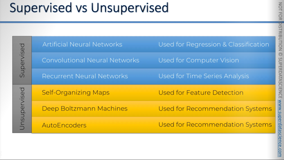
Deep Learning is the most exciting and powerful branch of Machine Learning. Deep Learning models can be used for a variety of complex tasks:

• ANN for Regression and Classification

• CNN for Computer Vision

• Recurrent Neural Networks for Time Series Analysis

• Self Organizing Maps for Feature Extraction

• Deep Boltzmann Machines for Recommendation Systems

• Auto Encoders for Recommendation Systems

In this part, you will understand and learn how to implement the following Deep Learning models:

1. Artificial Neural Networks for a Business Problem

2. Convolutional Neural Networks for a Computer Vision task

Let’s start!

What is Deep Learning?

About 25-30 years ago, people didn't know what the internet was. Now, we can't imagine a day without it!

However, I’ll be giving you a quick run on what is deep learning.

This is a photo of a computer from 1980. Neural networks and deep learning was invented back at 60s. But they got recognition in the 80s. People started talking about them, conducted a lot of researches and so on. They thought it will change the whole world but then the hype kind of died.

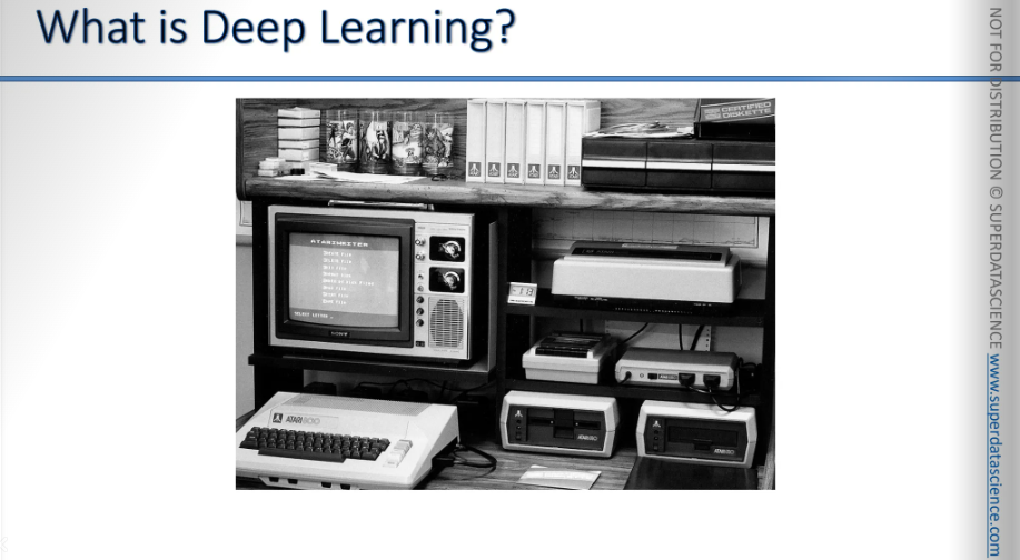
The technology to facilitate neural networks were not on the right margin. For deep learning and neural networking you need two things: enormous amount of data and strong processing power; which was not available back at that time.

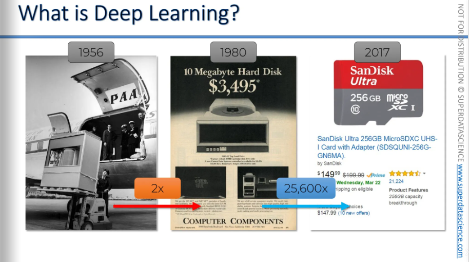
Here we have there years: 1956, 1980, 2017

How did storage look back in 1956? Well, there's a hard drive, and that's 5 megabytes right there. It's on a forklift, about the size of a small room. It was being moved to another location on a plane. In 1956. A company had to pay 2,500$ of that time's money to rent that hard drive for one month, not buy it, just rent it.

In 1980, the situation had improved a little bit. Still very expensive for only 10 megabytes (which is like one photo these days)

And in 2017, we've got a 256 gigabyte SSD card for $150, which can fit on your finger.

So from 1956 to 1980, storage capacity doubled, and then it increased about 25,600 times by 2017. The time periods aren't very different, but there was a huge leap in technology. This shows that the growth isn't linear; it's exponential.

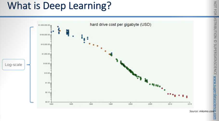
Here's a chart on an algorithmic scale. If we plot hard drive costs per gigabyte, it quickly approaches zero. Now, you can get free storage on Dropbox and Google Drive.

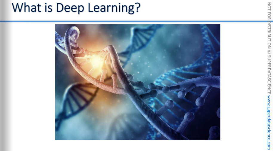
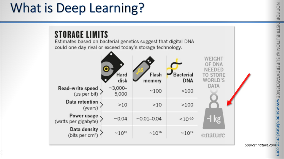
Currently, scientists are exploring the use of DNA for storage, although it's quite expensive. It costs $7,000 to synthesize 2MB of data and another $2,000 to read it.

This situation is similar to the early days of hard drives and planes. This is going to improve rapidly due to the exponential growth curve. Ten or twenty years from now, everyone will be using DNA storage.

This is from nature.com You can store all the world's data in just 1 kilogram of DNA storage. Alternatively, you can store about 1 billion terabytes of data in just 1 gram of DNA storage.

This example shows how fast we're progressing, which is why deep learning is gaining momentum now.

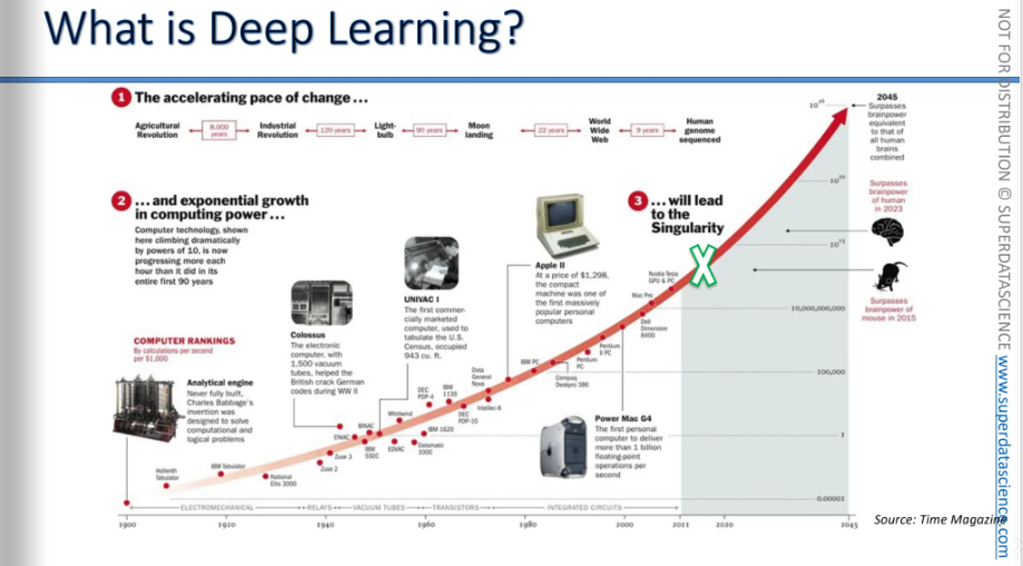
The same growth applies to processing capacity, which is also increasing at an exponential rate. This is known as Moore's Law, and you've probably heard of it.

Right now, computers have surpassed the thinking ability of a rat. They have already exceeded the thinking capacity of a human brain, and by 2040 or 2045, they will surpass the combined thinking power of all humans. So, basically we're entering the era of computers that are incredibly powerful and can process things much faster than we can imagine and this is what exactly facilitating the deep learning.

Now all of this makes us question: What exactly is deep learning? What is neural networking? what is it? What is going on here?

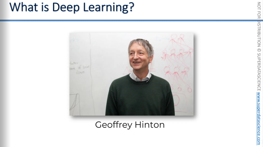
This gentleman, Geoffrey Hinton, is known as the godfather of deep learning. He conducted research on deep learning in the 1980s and has done a lot of work in the field. He has published many research papers on deep learning. Currently, he works at Google, so much of what we will discuss comes from Geoffrey Hinton. He won the 2024 Nobel Prize in Physics

He has many great YouTube videos where he explains things clearly, so I highly recommend checking them out.

The idea behind deep learning is to look at the human brain. It tries to mimic the brain (neuroscience stuff).We don't know everything about the human brain, but with the little we do know, we try to mimic it. Why? Because the human is one of the most powerful learning tool on this planet The way brain learns, adapts skills and apply them - we want our computers to copy that.

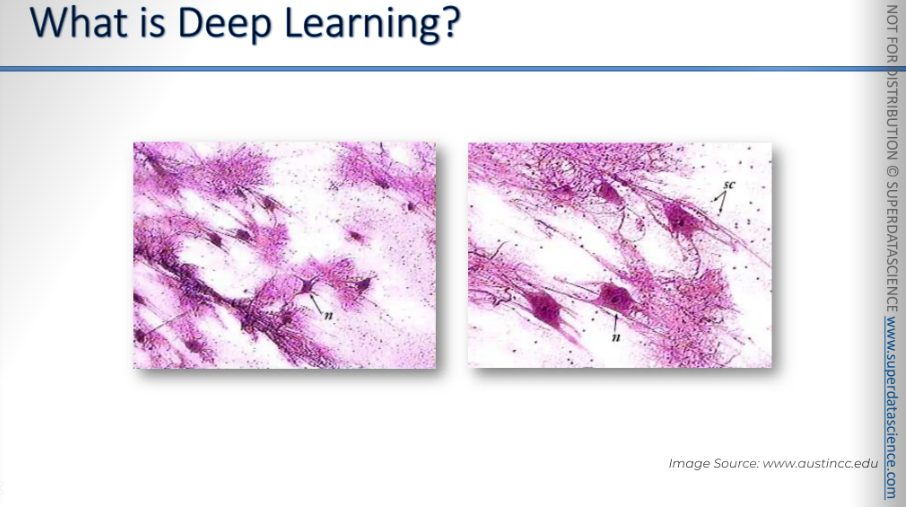
Here we have some neurons. These neurons are spread onto glass and observed under a microscope with some coloring. You can see what they look like. They have a body, branches, and tails. You can also see a nucleus in the middle. That's what a neuron looks like. In the human brain, there are approximately a hundred billion individual neurons in total and they are connected with each other.

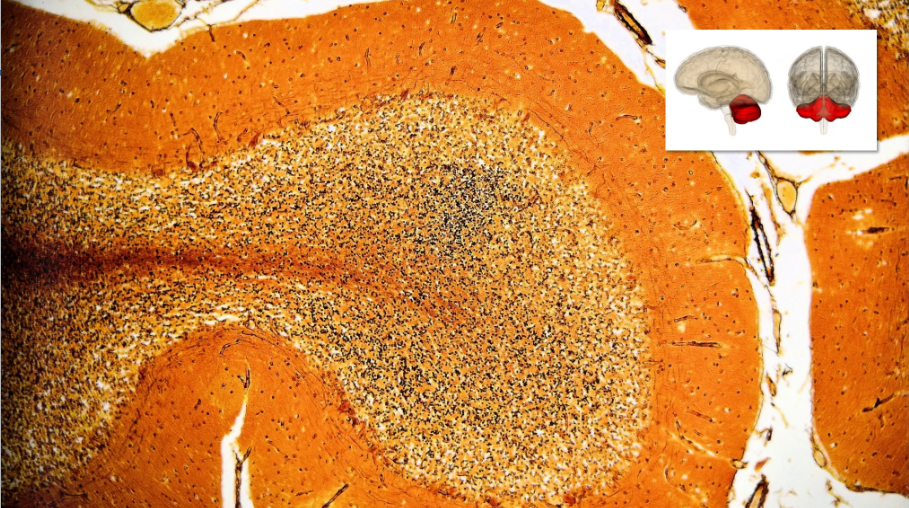
So to give you a picture of this, this is what it looks like, this is an actual dissection of the human brain.

This is just to show how vast the network of neurons is. There are billions and billions of neurons all connected in your brain. We're not talking about five hundred, a thousand, or even a million. We're talking about billions of neurons who takes care of memorizing, balancing etc. And yes, that's what we're going to try to recreate.

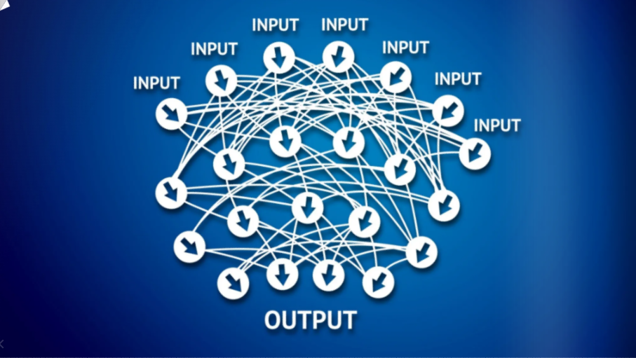
So how do we recreate this in a computer? We create an artificial structure called an artificial neural network.

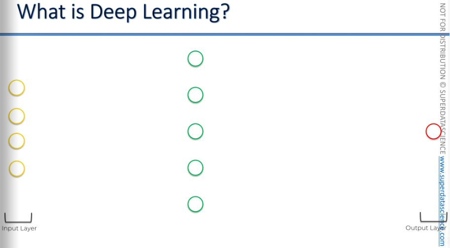
We have nodes or neurons, which are used for input values. These are the values you know about a certain situation. For example, if you're modeling something and want to make predictions, you'll need some input to begin with. This is called the input layer.

Then you have the output, which is the value you want to predict. This is called the output layer.

And in between, we have a hidden layer. In your brain, information comes through your senses like eyes and ears. It doesn't go straight to the result; it passes through many neurons first. This is why we use hidden layers in modeling the brain before reaching the output. This is the whole concept behind it: we are going to model the brain, so we need these hidden layers before the output.

Neurons are connected to the hidden layer, and the hidden layer is connected to the output value.

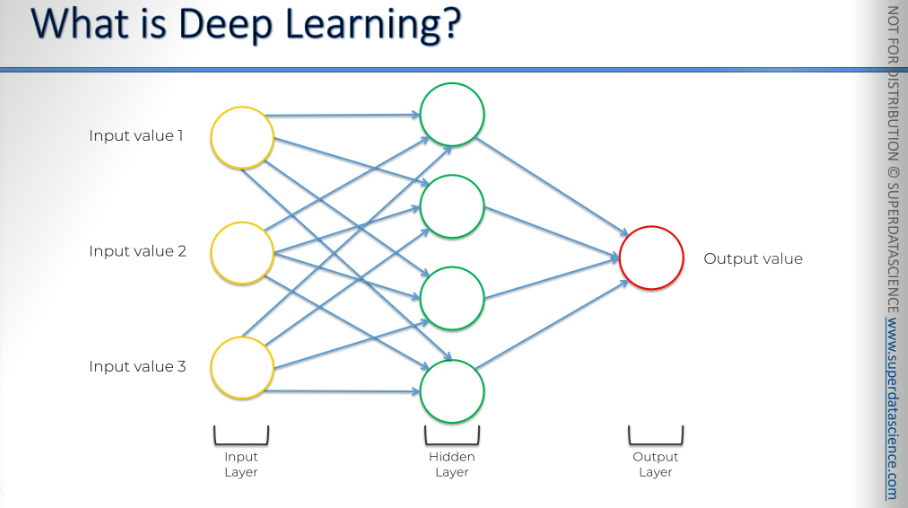
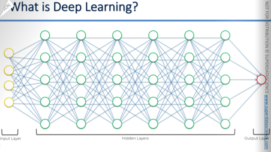
And then we connect everything, just like in the human brain. Connect everything, interconnect everything. That's how the input values process through all these hidden layers, just like in the human brain, and then we get an output value.

This is what deep learning is all about at a very abstract level.

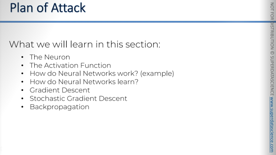
Plan of attack

The are the topics we will learn in this blog

(This is something to worth remember)

The Neuron

I hope you have seen the neuron references. We need to create a structure like that cause this is the whole point of deep learning: mimicking the brain.

So our first task is to recreate a neuron.

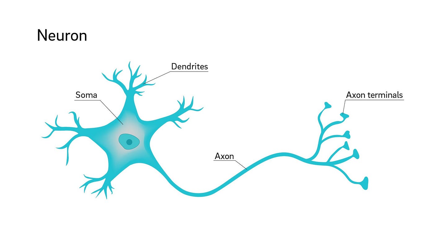
This is what a neuron looks like, it got a body, some branches on top (dendrites), a long tail (Axon). But a single neuron is useless. It’s not functional by it’s own. But if a lot of them works together, they do magic. And do you know how they work together? Neurons connects with each other through their branches aka Dendrites and Axon terminals. Dendrites works like a receiver, Axon works like a transmitter.

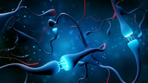
This is an image of them doing it. Dendrites are connected with axons of other neurons That’s how they stay connected with each other and pass signal in a form of electrical impulses.

As you can see, the axon doesn't actually touch the dendrites. The connection between them, where the signal is passed, is called the synapse. Instead of calling our artificial neuron connectors axons or dendrites. To avoid confusion - we'll just call them synapses.

Let’s dig deeper!

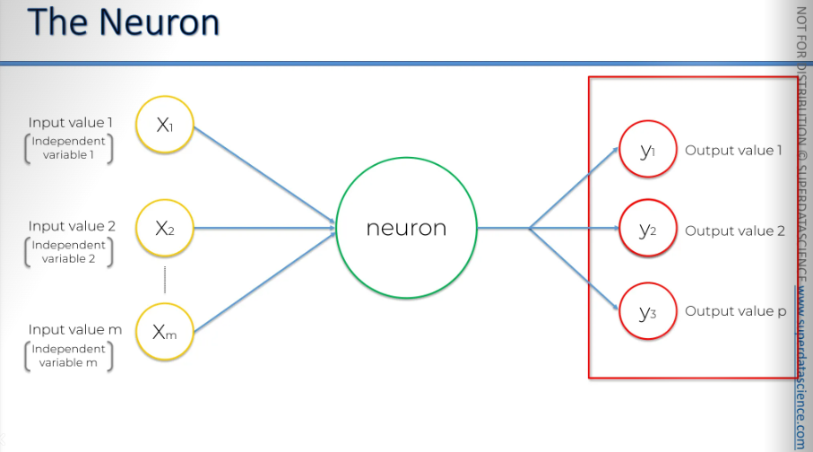
The neuron is also called a Node. The neuron gets some input signals and it has an output signal.

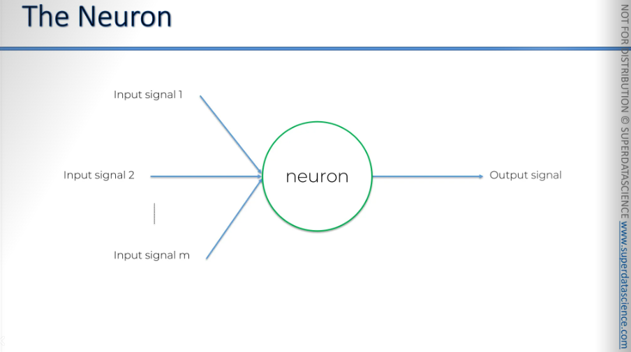
These input signals show that the green neuron is receiving signals from the yellow neurons. (In this blog, we'll use a color-coding system where yellow represents an input layer) What I want to highlight here is that, in this example, we're looking at a neuron receiving signals from the input layer neurons. These are also neurons, but they belong to the input layer. Sometimes, you'll have neurons that get their signals from other hidden layer neurons, which are the other green neurons.

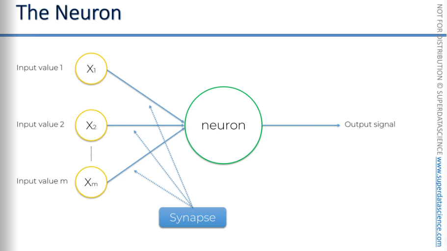
The signal is passed through synapses to the neuron, and then the neuron has an output value that it sends further down the chain. So yah this is the basic picture.

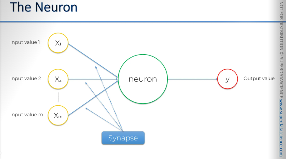
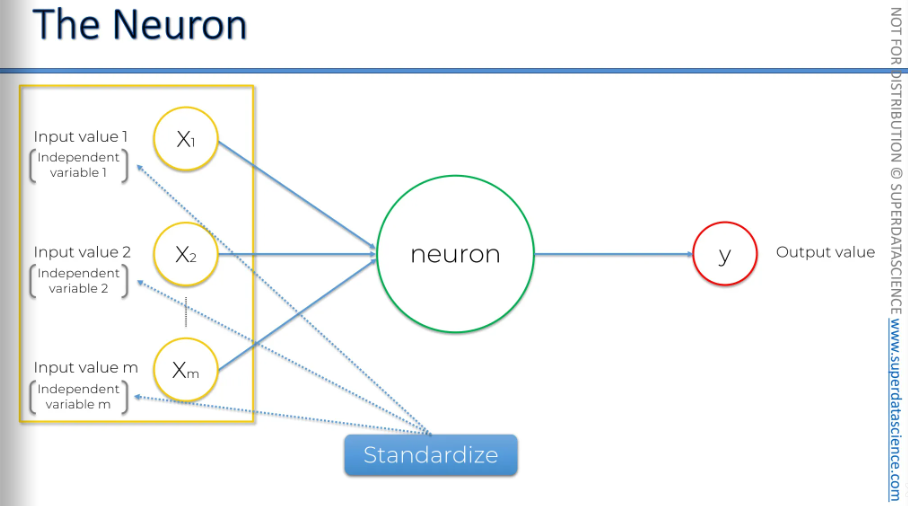
Now let's take a closer look at these elements. We have the input layer, and what do we have here? Well, we have these inputs, which are actually independent variables: independent variable 1, independent variable 2, up to independent variable m.

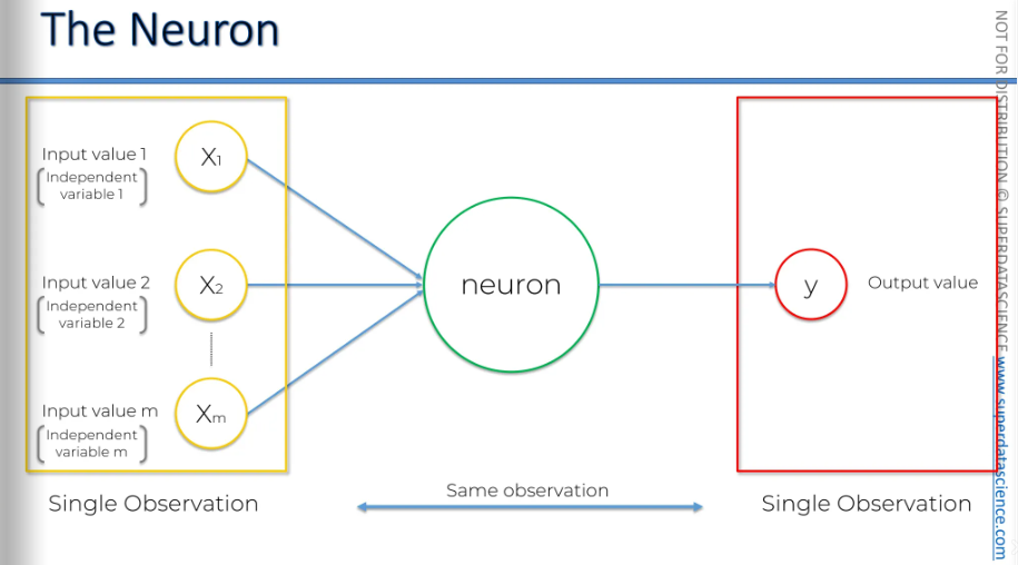
The important thing to remember is that these independent variables are all for a single observation. Think of it as just one row in your database. One observation (could be age, salary and gender of a person)

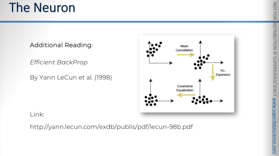
Another important thing to know about these variables is that you need to standardize them. This means ensuring they have a mean of zero and a variance of one. Alternatively, you can normalize them, which I will explain in detail in the practical section.

Whatever we do, we need to make them similar cause it will be easier for our neural network to compute them if they are similar.

If you want to learn more about standardization, normalization, and other techniques for your input variables, a good resource is the paper "Efficient Backprop" by Yann LeCun, 1998. You can find it here: Efficient Backprop. [Yann LeCun is a remarkable figure in the field of deep learning. We'll discuss him more in the section of the course about convolutional neural networks. He is a close friend of Geoffrey Hinton]

Here we have the output value. The output value can be continuous, like a price. It can also be binary, such as whether a person will exit or stay. Additionally, it can be a categorical variable.

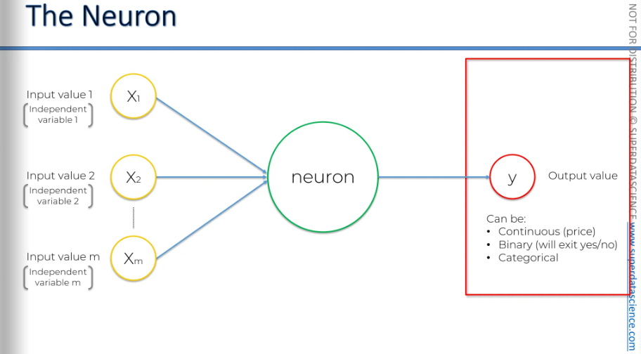
If it's categorical, remember that your output value won't be just one; there will be several output values. These will be your dummy variables representing the categories. That's how it works.

Let's go back to a simple case with one output value. On the left, you have a single observation from your dataset, and on the right, you have the same observation. It's important to remember that when you're training your neural network, you're inputting the data for one row and getting the output for that same row. To simplify the complexity, think of it like a simple linear regression or a multivariate linear regression.

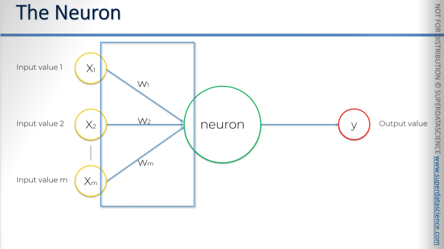
Next: the synapses. Synapses have assigned weights, and neural networks learn by adjusting these weights. The neural network determines, in each case, which signals are important and which are not for a particular neuron.

When you're training an artificial neural network, you're basically adjusting all the weights in all the synapses throughout the whole network. That's where gradient descent and backpropagation come in handy. Anyway we’ll talk about this later in this blog.

Now - what happens inside the neuron?

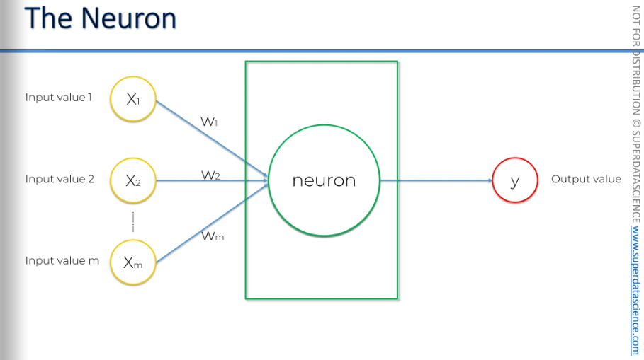
The first thing that happens is: all of the values gets added up inside the neuron. Vey straightforward.

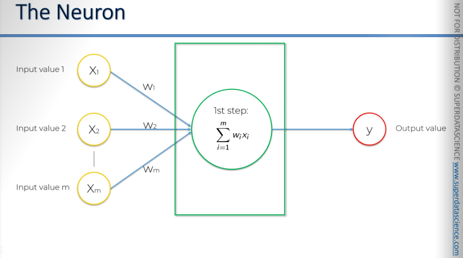
Then it applies an activation function on the summation. Basically, this function is assigned to the neuron or, the whole layer from which the neuron understand if it needs to pass the signal (information) or not.

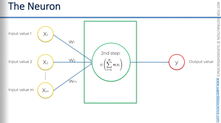
And that's exactly what happens here in step three: the neuron passes the signal to the next neuron in the sequence.

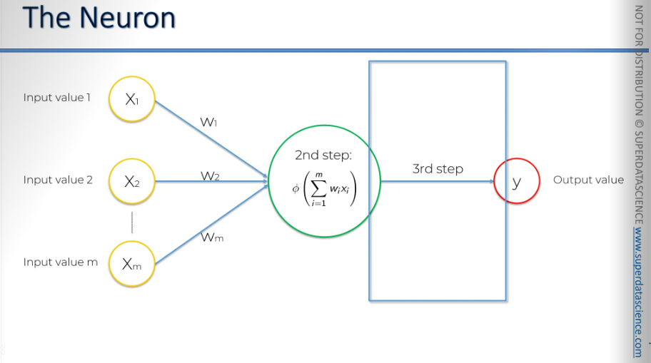
The Activation Function

Alright, we know it has inputs and weights. It adds up the weighted inputs, applies the activation function, and then passes the signal to the next neuron. And now I’ll explain

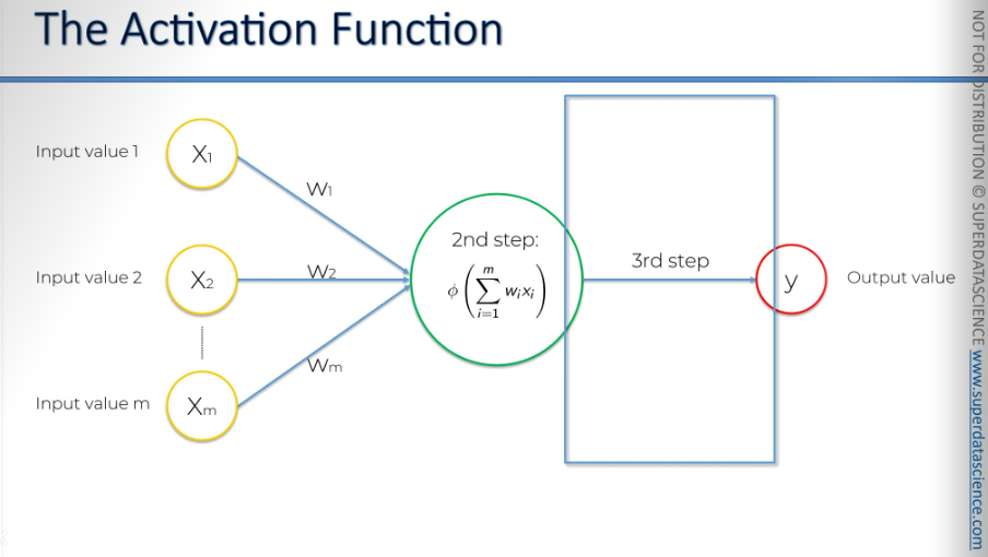
We have four types of activation functions to choose from. There are more but there 4 are the dominant one.

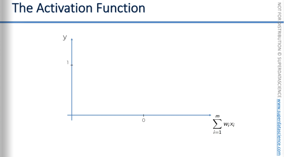
Here is the Threshold function.

This is what it looks like: on the X-axis, you have the weighted sum of inputs, and on the Y-axis, you have values from zero to one. The threshold function is a very simple type of function. If the value is less than zero, the threshold function outputs 0. If the value is greater than or equal to zero, the threshold function outputs 1.
So, it's basically a yes-or-no type of function. It's very straightforward and quite rigid, offering no other options.

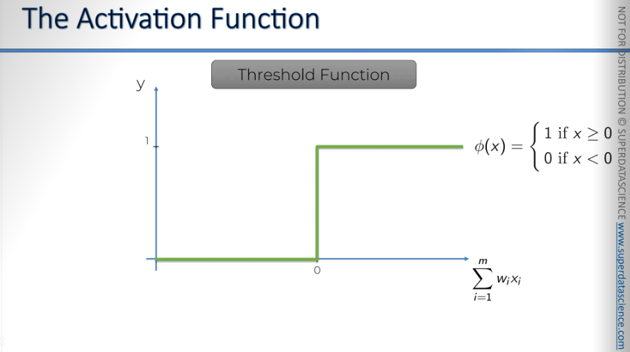
Let's move on to the Sigmoid function.

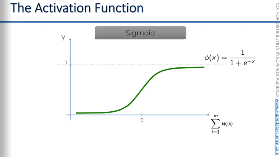
One divided by one plus e to the power of -x.

Here, x is of course, the value of the weighted sums. This function is used in logistic regression, as you might remember from the machine learning course, the advantage of this function is that it is smooth.

Anything below zero drops off, while above zero, it approaches one. This sigmoid function is very useful in the final layer, the output layer, especially when you are trying to predict probabilities.

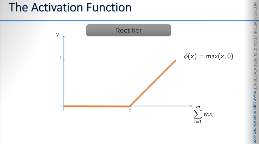
The Rectifier function, one of the most popular and used function in neural networks. Basically, it starts at zero and remains zero. Then, as the input value increases, it gradually rises.

The Hyperbolic Tangent Function.

It's very similar to the sigmoid function, but the hyperbolic tangent function goes below zero. The values range from approximately one to minus one. This is useful in some applications.

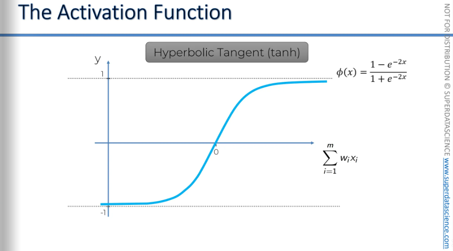
Now i’m not going in depth with these functions. I just gave an basic idea of them. But if you wanna acquire more knowledge, then check out this paper by Xavier Glorot.

Now I have a question: assuming your dependent variable is binary, which activation function will you choose, threshold or sigmoid?

The first option is the threshold activation function. It outputs either zero or one, depending on certain values, which fits this requirement perfectly. You can simply say y equals the threshold function of your weighted sum, and that's it.

The second option is the sigmoid activation function. It also ranges between zero and one, which is what we need. However, if you want just zero or one, instead, you can use it to find the probability of y being yes or no. We want y to be zero or one, but the sigmoid function tells us the probability of y being equal to one. Basically, the closer the output is to one, the more likely it is to be a yes rather than a no. This is very similar to the logistic regression approach. These are just two examples for when you have a binary variable.

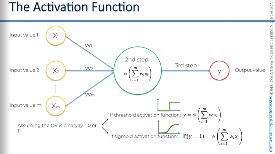
Let's see how this would work if we had a neural network like this.

In the first input layer, we have some inputs. They're sent to the first hidden layer, where an activation function, usually the rectifier, is applied. Then, signals go to the output layer, where the sigmoid activation function is applied, giving us the final output, which could predict a probability.

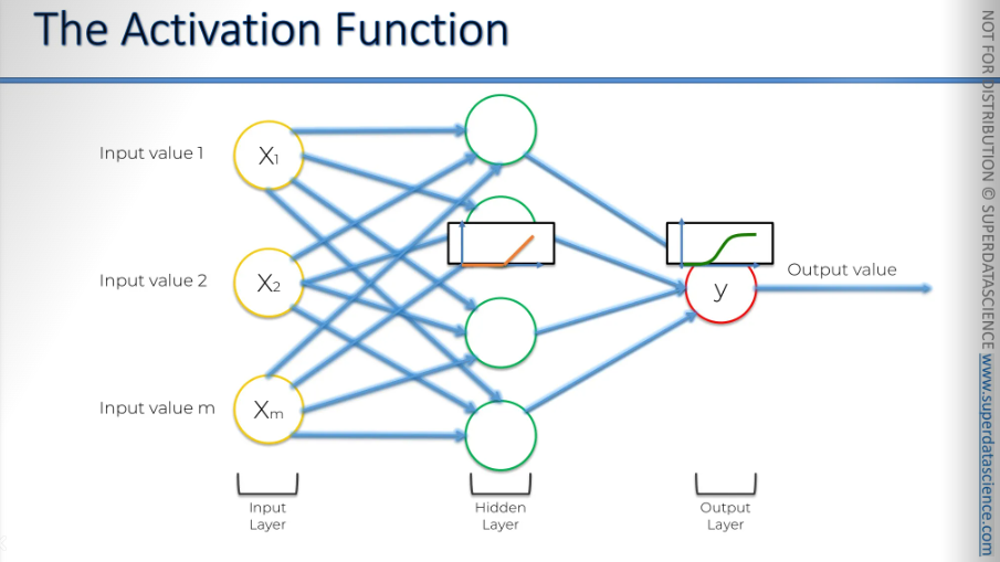
This combination is quite common.

How do Neural Networks work?

To learn how a neural network works, we are going to look at property valuation. We'll examine a neural network that takes in some parameters of our property and evaluates it. By the way, we're not actually going to train the network.

Let’s say we have 4 input parameters about the property. There’s no hidden layer here, only the input and output parameter.

These input variables are weighted by the synapses, and then the output is calculated, giving us a price. We can use almost any function here. We could use any of the activation functions we mentioned earlier, like logistic regression or a squared function. You can use just about anything. The main point is that you get a specific output.

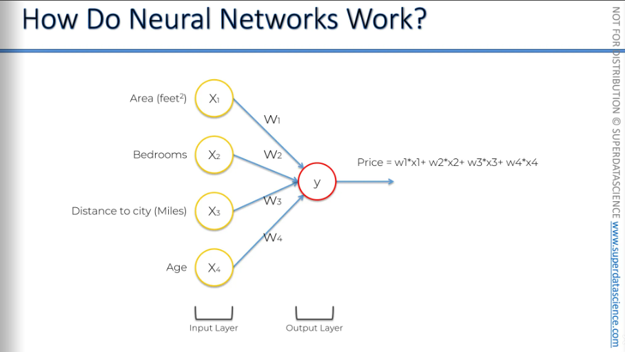
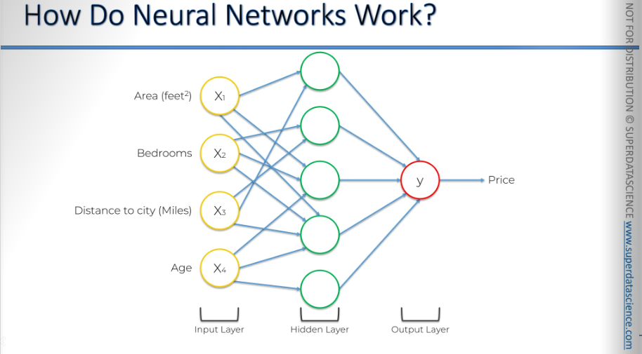
But in neural networks, we have an extra benefit that gives us a lot of flexibility and power, which boosts accuracy. This power comes from the hidden layers. And there it is, our hidden layer, we've added it in.

All right, we have all four variables on the left, and we'll start with the top neuron in the hidden layer. These synapses have weights. Let's agree that some weights will have a non-zero value, while others will have a zero value, because certainly, not all inputs will be valid, or not all inputs will be important for every single neuron. Sometimes inputs will not be important.

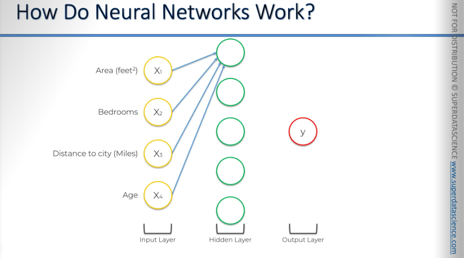
Here, we see two examples: X1 and X3, which are the area and distance to the city, are important for that neuron, while bedrooms and age are not. This makes sense, right? The price depends on how far the house is from the city. So, this neuron is specifically picking out those properties and will activate only when certain criteria are met. It performs its own calculation, and when it activates, it contributes to the price in the output layer.

Therefore, this neuron doesn't really care about the number of bedrooms or the age of the property because it's focused on those specific factors.

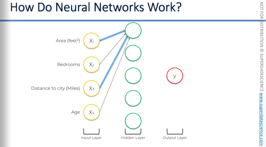
Here, we have three parameters feeding into this neuron: the area, the number of bedrooms, and the age of the property.

What could be the reason here? Let’s try to understand the intuition here.

We've established this is a trained dataset. The training happened a while ago, or someone has already trained it. Now, we're applying it, and we know this neuron has learned from many property examples that the combination of area, bedrooms, and age is important. Why might that be?

For example, in the specific city and its suburbs where this neural network was trained, there might be many families with two or more children looking for large, new properties with lots of bedrooms. These families prefer newer properties because, in that area, big properties are often older. There might have been a demographic shift, or perhaps there has been growth in job opportunities for younger people. As a result, younger couples or families now seek newer properties.

Therefore, this neural network has learned from its training that properties with a large area and many bedrooms—at least three for the parents and children, and maybe a guest room—are valuable in that market. The neuron has recognized this pattern and knows what to look for.

It doesn't care about the distance to the city in miles, as long as the property has a large area and many bedrooms. Once these criteria are met, the neuron activates.

The power of the neural network comes from combining these three parameters into a new attribute that helps evaluate the property more precisely.

So, that's how this neuron works.

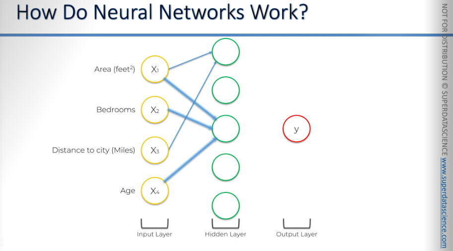
Let’s consider another example. This neuron might have focused on just one parameter, such as age, without considering the others. How could that happen?

Alright, so here's a classic case of how age can play a role. We all know that older properties usually aren't as valuable because they're worn out, the building's old, and things might be falling apart, needing more maintenance. So, the price tends to drop. On the flip side, a brand new building is pricier because, well, it's new.

But here's the twist: if a property is over a certain age, it might actually be a historic gem. For example, if a property is under 100 years old, the older it gets, the less valuable it is. But once it hits that 100-year mark, bam, it becomes historic. It's like, "Hey, people lived here ages ago!" It's got stories and history, and some folks really dig that. In fact, lots of people love that and would be super proud to live in such a place. Especially those in higher social circles—they'd totally show it off to their friends.

So, properties over 100 years old can be seen as historic, and when this neuron spots one, it lights up and boosts the price. But if it's under 100 years, it doesn't even bother. This is a good example of how the rectifier function being applied. So, you've got a zero until 100 years old, and after that, the older it gets, the more it contributes to the price.

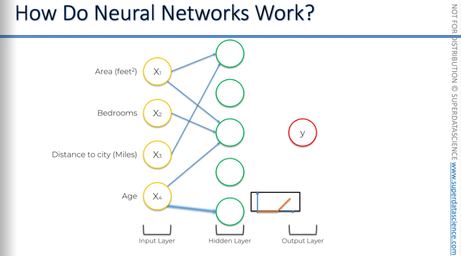
Moreover, the neural network might identify factors we wouldn't consider, like how bedrooms and distance to the city together affect the price. It might not be as influential as other factors, but it still plays a role, either increasing or decreasing the price.

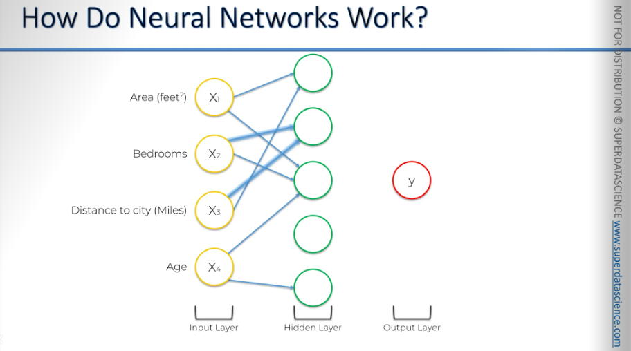
And maybe a neuron picked up a combination of all four of these parameters.

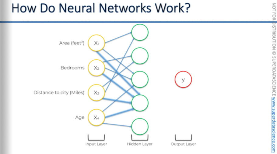
As you can see, these neurons and the hidden layer setup let you make your neural network more flexible. This allows the neural network to look for very specific things. And then it combines all of them, from where the real power comes from.

It's like an example of ants. A single ant can't build an anthill, but when you have 1,000 or 100,000 ants, they can build an anthill together. And that's the situation here: each neuron alone can't predict the price, but together they have the power to do so accurately if trained and set up properly.

How do Neural Networks learn?

Now that we've seen neural networks in action, it's time for us to find out how they learn.

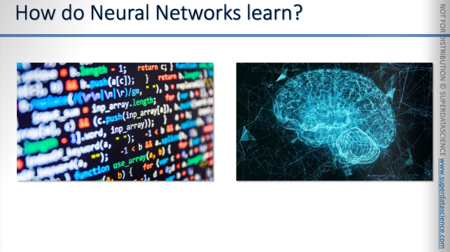
There are two main ways to make a program do what you want. One is hard coding, where you give the program specific rules and guide it completely. The other is using neural networks, where you enable the program to learn and understand on its own. Our goal here is to create a network that learns on its own. We will avoid putting rules as much as we can.

For example, how do you tell the difference between a dog and a cat?

With hard coding, you would program specific details, like the cat's ears need to look a certain way,

• Look out for whiskers.

• Look out for this type of nose.

• Look out for this type of shape of face.

• Look out for these colors.

You describe all these features and set conditions, like if the ears are pointy, then it's a cat. If the ears slope down, then it might be a dog, and so on.

On the other hand, with a neural network, you simply program the network's architecture. Then, you direct the neural network to a folder containing images of cats and dogs that are already categorized.

And you tell it, Okay, I've got some images of cats and dogs.

• Go and learn what a cat is.

• Go and learn what a dog is.

The neural network will independently learn everything it needs to know. Later, once it's trained, when you give it a new image of a cat or a dog, it will be able to recognize what it is.

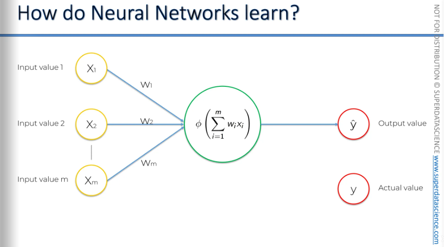
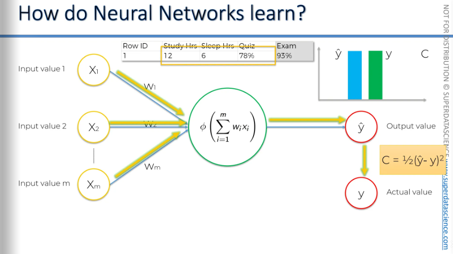
This is known as a single-layer feedforward neural network, also called a perceptron. Before we proceed, it's important to clarify the output value. We use "y hat" here. Usually, "y" stands for the actual value we see in real life, and "y hat" represents the predicted value, calculated by the neural network.

The perceptron was first invented in 1957 by Frank Rosenblatt. His main idea was to create something that could learn and adjust itself.

Okay, let's say we have some input values provided to the perceptron, or basically to our neural network. Once the activation function is applied, we get an output. Now, we're going to plot the output on a chart.

To learn effectively, we need to compare the output value to the actual value we want the neural network to achieve, which is the value y. If we plot it on the chart, you'll notice there's a slight difference. Now, we will calculate a function called the cost function. The cost function tells us what is the error in our prediction. Our goal is to minimize the cost function. The lower the cost function , the closer is y hat to y.

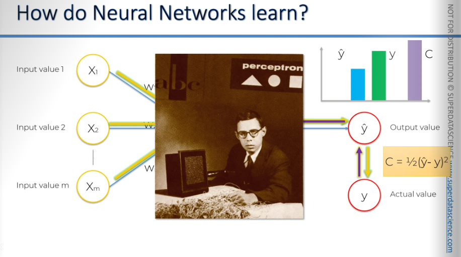
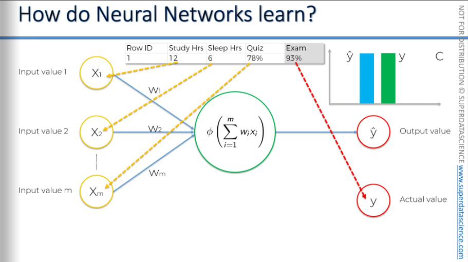
Let me remind you again, we are dealing with one row. Here, we have some variables, and based on these variables, we're trying to predict the score you'll get on the exam. In the exam, the 93% is the actual value, which is y.

Now, we feed these values into the neural network, and everything gets adjusted, including the weights. And then we're going to be comparing the result to y.

Once we have compared, we are going to feed this information back into our neural network (the purple arrow is indicating information going back) The only thing we have control over here are the weights.

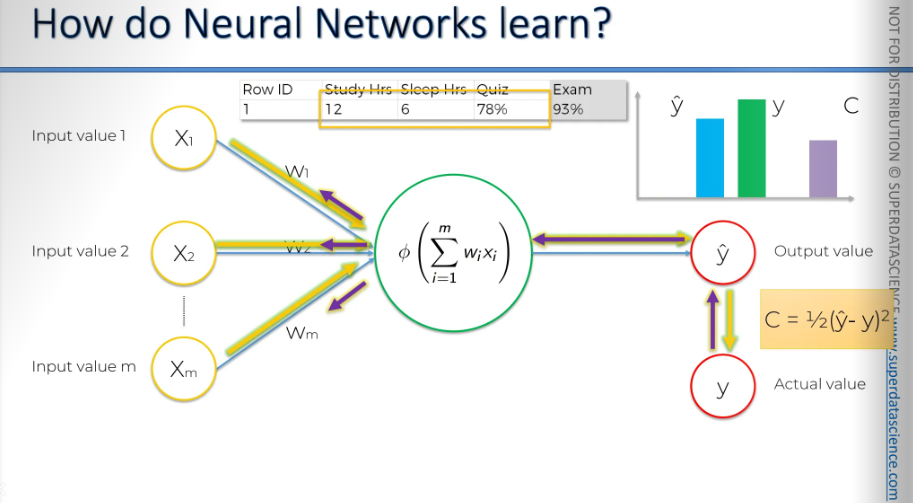
So again, we feed these rows in.

Our cost function gets adjusted.

As you can see, everything follows the same process. Every time our y-hat changes, because we've adjusted the weights, our y-hat changes, and our cost function changes.

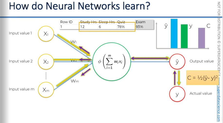
Let's do this again.

We feed the data in. Y-hat changes, and the cost function changes. We receive information back, which adjusts the weights again.

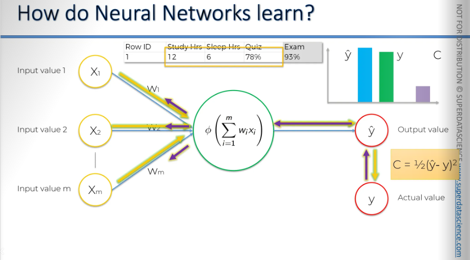
We input the same values each time. Everything gets adjusted, the adjustments go back to the weights.

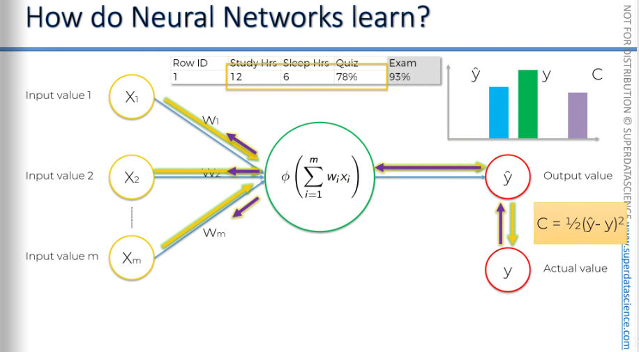
And one more time. We feed in, okay?

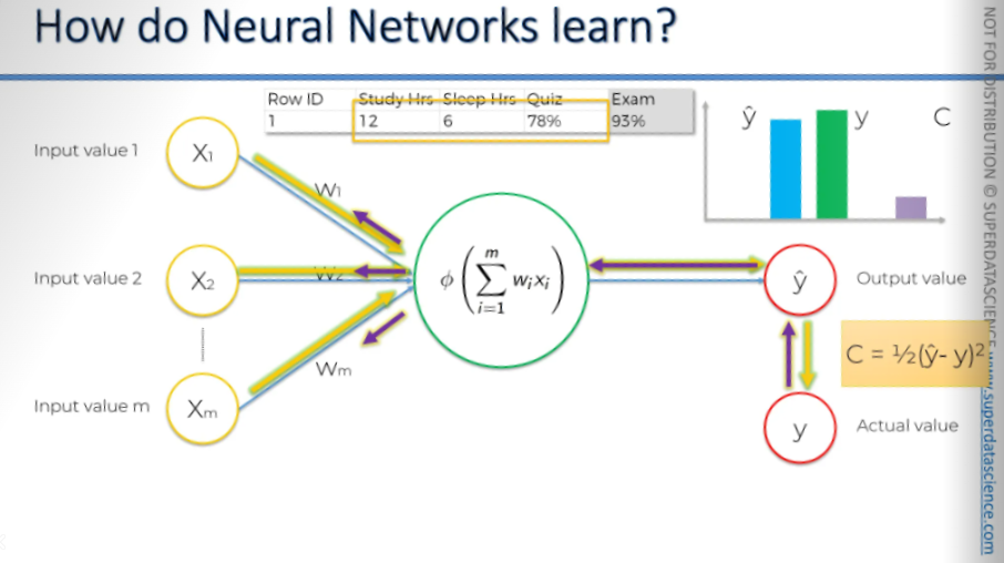
And once more. We've adjusted the weights. We feed in the information, and there we go. A-ha! This time, y-hat is equal to y, and the cost function is zero. Usually, you won't get a cost function equal to zero, but this is a very simple example.

I hope that all made sense!

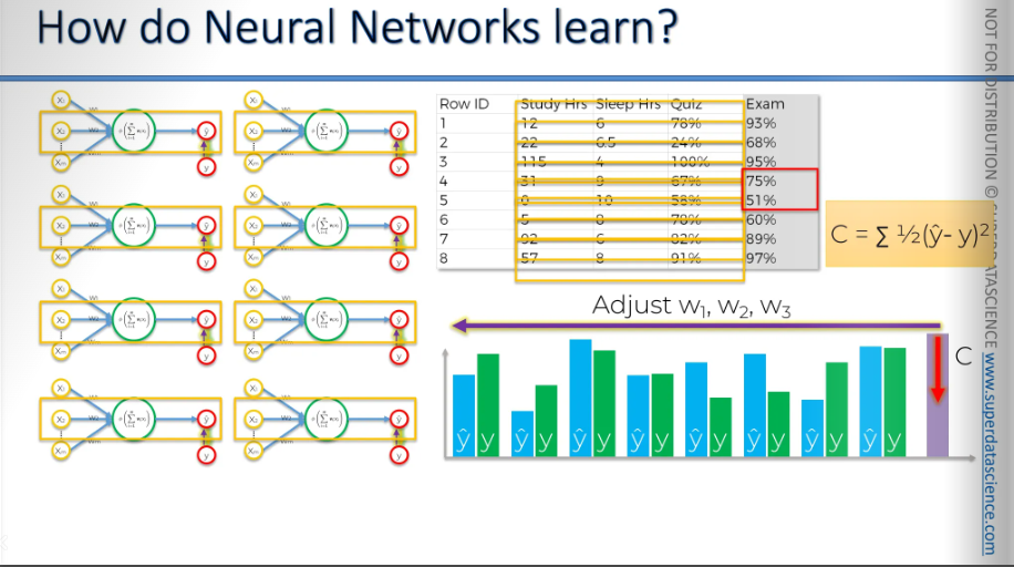
Let's see what happens when you have multiple rows of data. We have eight rows showing how many hours you slept, or maybe these are different students taking the same exam. It includes how many hours they studied, how many hours they slept before the exam, their quiz scores, and their final test results.

We're going to feed all this data into the same neural network.

Here's our first row. And here's y-hat for the first row. Here's the second row. And here's y-hat for the second row. Each time, it's fed into the same neural network. I've repeated them several times so we can see how this works. And it happens again. Here's the third row, the fourth row. And here's y-hat for the fourth row, and so on.

Basically, we get the same values for the remaining four rows as well. Each time we feed a row into our neural network, we get a value. Then we compare it to the actual values. The green bars represent the actual values. For each row, there is an actual value. Now, based on the differences between y-hat and y, we can calculate the cost function.

After we have the complete cost function, we go back and update the weights. We update W1, W2, and W3. The important thing to remember here is that all these perceptron, all these neural networks, are actually part of one neural network. So, there aren't eight separate networks; there's just one. And when we update the weights, we will update them in that single neural network. So it's not the case that every row has its own weights.

This is just one iteration. Next, we're going to run this whole thing again.

We will feed each row into the neural network, determine our cost function, and repeat this process for every row in your dataset. After completing this process, you calculate the cost function in order to achieve one goal: find minimum cost function. As soon as possible you find the minimum cost function, that is your final neural network. This whole process is called backpropagation.

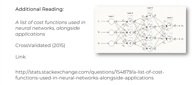
Some additional reading: A list of cost functions used in neural networks, alongside applications. It actually has some good stuff in it.

Gradient Descent

Here we are going to learn how the weights are adjusted.

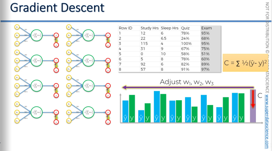
This is our basic version of a neural network—a perceptron or a single-layer feed-forward neural network. Here, we can see the entire process in action. We start with an input value, apply a weight, and then an activation function. We get y-hat and compare it to the actual value to calculate the cost function. So, how can we minimize the cost function?

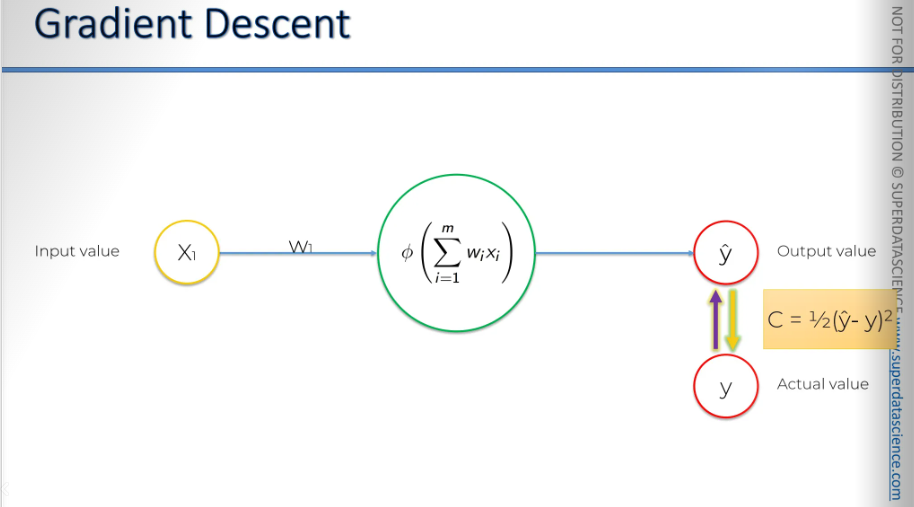
One way to do this is by using a brute force method. We try many different weights to see which one works best. For example, we could test a thousand weights. This would give us a curve for the cost function. On the Y-axis (vertical), we have the cost function, and on the X-axis (horizontal), we have Y hat. Since the formula is Y hat minus Y squared, the cost function would look like a parabola. We find the best weight where the cost is lowest.

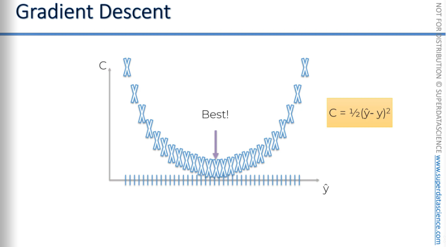
Well, if you have just one way to optimize, this might work. But as you increase the number of weights and synapses in your network, you will encounter the curse of dimensionality. So, what is the curse of dimensionality?

Let’s understand this with an example: Remember when we talked about how neural networks actually work, like when we built or ran a neural network for property valuation? This is what it looked like once it was fully trained, right?

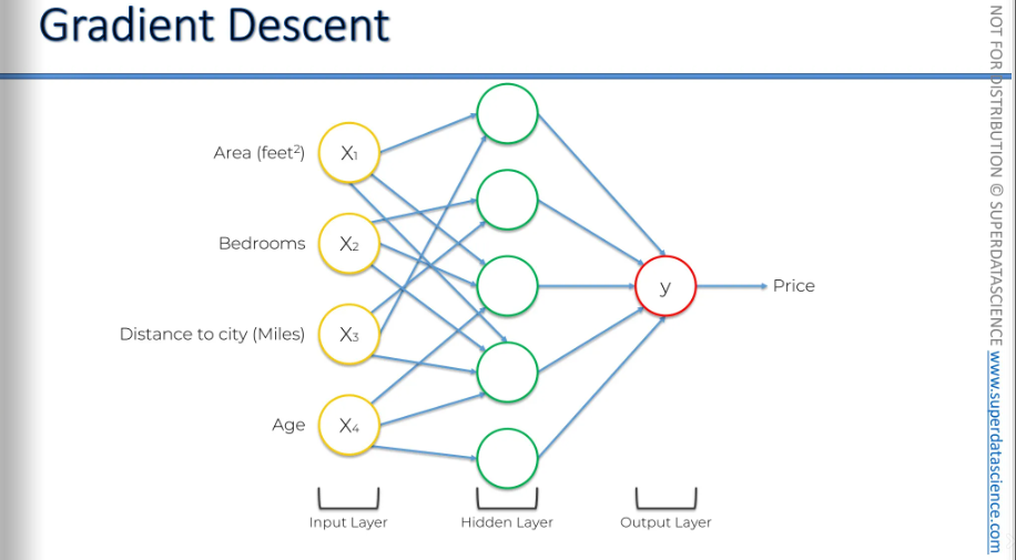
When the neural network is not yet trained, it looks like this. We have many possible synapses, and we still need to train the weights.

Here, we have a total of 25 weights. That's four times five at the start, plus five more from the hidden layer to the output layer, making 25 weights in total.

Let's see how we could possibly use brute force to find the best 25 weights. This is a very simple neural network. It has just one hidden layer. How could we use brute force to work through a neural network of this size?

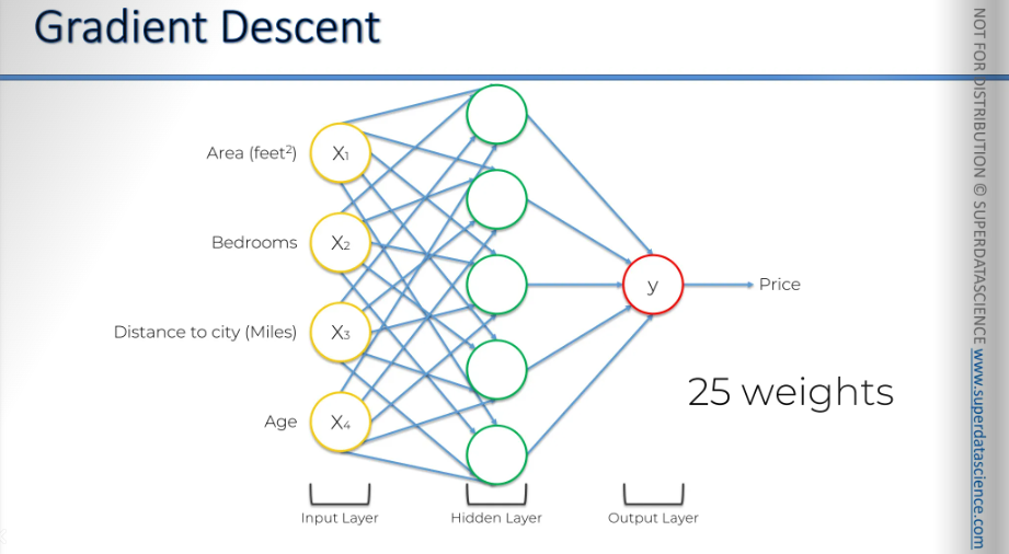
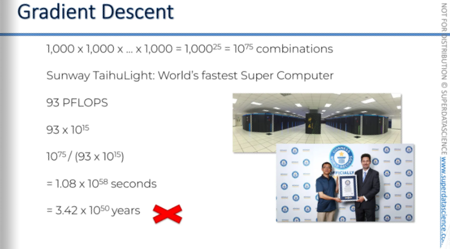
Let's do some math. If we test 1,000 combinations for each weight, there are 10^75 total combinations. Now, let's see how Sunway TaihuLight, the world's fastest supercomputer as of June 2016 - 2018, would approach this problem. Sunway TaihuLight operates at 93 petaflops, meaning it can perform 93 x 10^15 floating operations per second [Flop stands for floating operation per second]

Let's say, hypothetically, it could test one combination for our neural network in just one flop, which is one floating operation. This isn't possible in reality because testing a single weight in your neural network requires multiple floating operations. But let's imagine it could for a moment.

That means it would take 10^75 divided by 93 x 10^15 seconds to run all those tests, which is about 10^58 seconds, or 10^50 years. This is longer than the universe has existed! Brute force is simply not going to work for us to optimize.

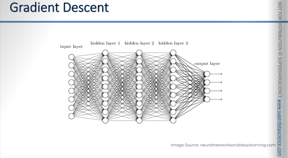
By the way, the neural network we calculated was a simple one What if our network looked like this?

So the method we’ll learn is gradient descent.

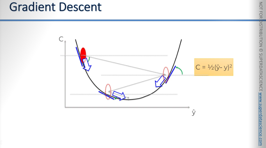
Here's our cost function. Let's say we start at a certain point. You have to begin somewhere, so we start there, in the top left. From that point, we'll examine the slope of our cost function. This is why it's called gradient, because you need to find the slope by differentiating. You need to differentiate to find out that the slope is in that specific location and find out if the slope is positive or negative.

if the slope is negative: you're going downhill. So, to the right is downhill, and to the left is uphill. This means you need to move to the right. Essentially, you need to go downhill, the ball rolls down (to the 3rd arrow).

Again, it's the same process. You calculate the slope. This time, the slope is positive, which means the right is uphill, and the left is downhill, so you need to move left. Then, you roll the ball down (from the 3rd arrow to the 2nd arrow, right to left)

And again you calculate the slope and you roll the ball.

In simple terms, that’s how you find the best weights, the best situation that minimizes your cost situation. It’s kind of like a zigzaggy type of method.

Instead of brute forcing, we can simply check which way the slope is going each time.

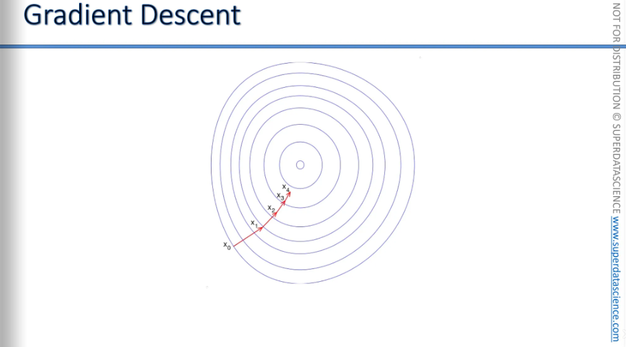
Imagine you're on a hill. You feel which way is downhill and walk that way. After 50 steps, check again which way is downhill. Then take 40 steps in that direction. The steps get smaller as you get closer.

This is an example of gradient descent in two dimensions. As you can see, it's getting closer to the minimum, which is why it's called gradient descent—because you're moving down towards the minimum of the cost function.

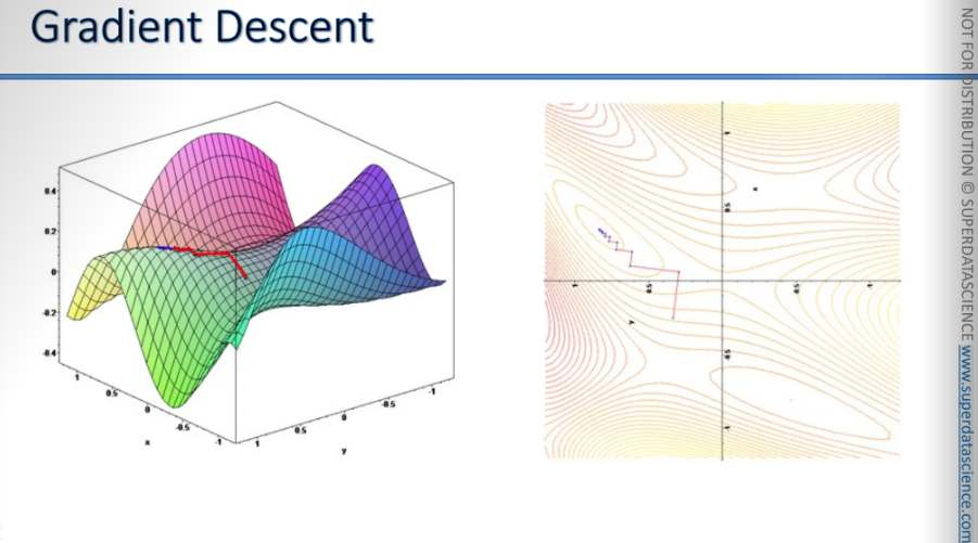
Finally, here's gradient descent applied in three dimensions. When you project it onto two dimensions, you can see it zigzagging its way toward the minimum.

Stochastic Gradient Descent

We learned that gradient descent is an efficient way to minimize the cost function, reducing problem-solving time from billions of years to minutes or hours. It speeds things up by showing the downhill direction, allowing us to reach the minimum quickly.

But the problem with gradient descent is, it requires for the cost function to be convex. Convex means the function curves in one direction, having one global minimum, which is what we aim to find.

But what happens if we encounter a function which is not convex?

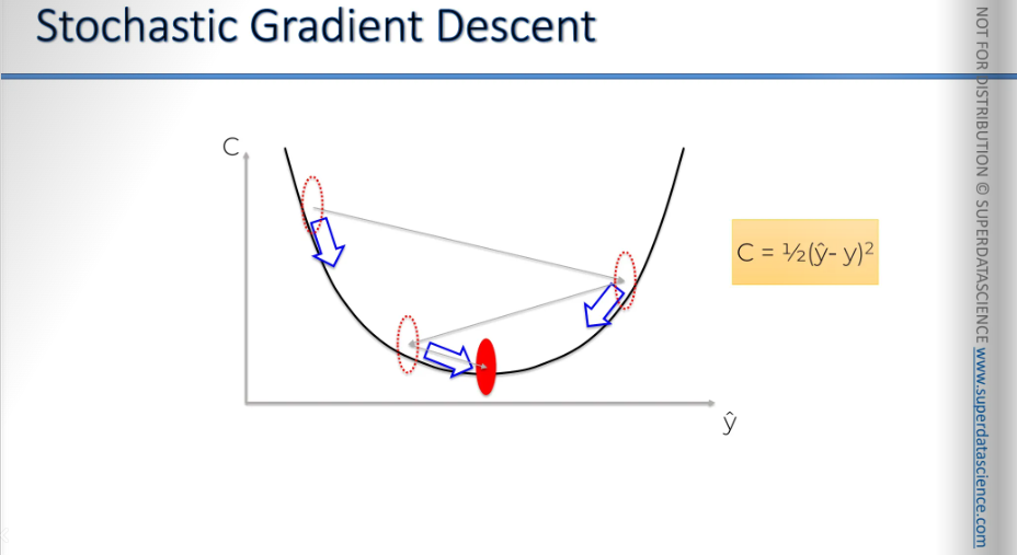
For example, like this? If we applied gradient descent to this type of function, as you can see, this could lead us to a local minimum instead of the global one(the red point). Therefore, we wouldn’t have the correct weight!

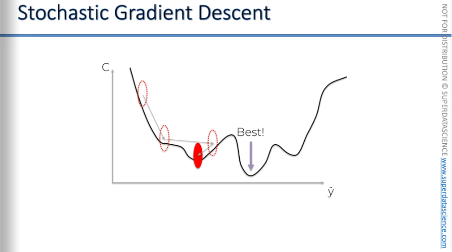
To solve this situation, we need stochastic gradient descent. Normal gradient is when we take all of the rows and plug them in our neural network. After plugging them, we calculate our cost function. And we adjust the weights by looking at the chart bellow. This is called the gradient descent method, or more precisely, the batch gradient descent method. We take the whole batch from our sample, apply it, and then run it.

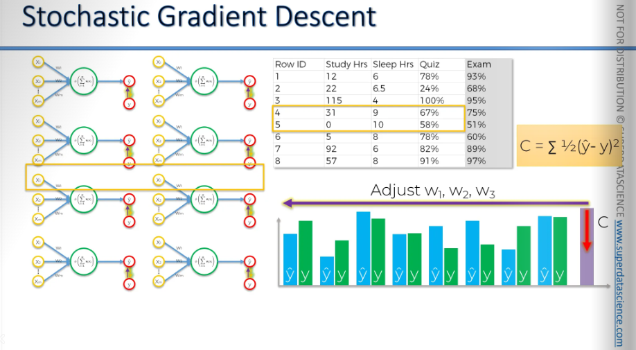
The stochastic gradient descent method works a bit differently.

Here, we process each row one by one.

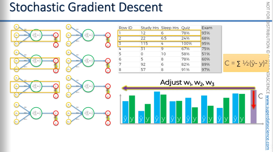
First, we take a row, run it through our neural network, and then adjust the weights. Next, we move to the second row.

We take the second row, run it through the neural network, check the cost function, and adjust the weights again. Then we proceed to the third row.

We run it through the neural network, check the cost function, and adjust the weights.

In essence, we adjust the weights after processing each row, instead of processing everything at once and then adjusting the weights.

Two different approaches, now let's compare them side by side.

Batch gradient descent

• So, with batch gradient descent, you adjust the weights after running all the rows through your neural network. Then, you adjust the weights and run the entire process again, repeating it for each iteration.

Stochastic gradient descent

• You process one row at a time and adjust the weights. You keep adjusting the weights after each row, and then you repeat the whole process over and over.

The two main differences are:

1. Avoiding Local Minima: Stochastic gradient descent helps avoid getting stuck in local minima. The stochastic gradient descent method has much higher fluctuations because it processes one row at a time. This means it can handle these fluctuations and is more likely to find the global minimum rather than just a local minimum.

2. Speed: Although it might seem slower since it handles one row at a time, stochastic gradient descent is actually faster. It doesn't need to load all the data into memory at once, so it can process each row individually, making it a lighter and quicker method.

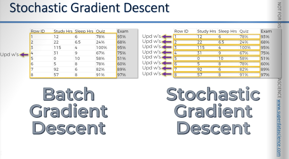
The main benefit of batch gradient descent is that it's predictable. Unlike stochastic gradient descent, which is random, batch gradient descent will always give the same results if you start with the same weights. This means the way your weights are updated will be consistent each time you run it.

With stochastic gradient descent, you won't have this consistency because it's random. You might pick rows randomly and update your neural network in a random way. So, even if you start with the same weights, each run will follow a different path and have different steps. That's basically what stochastic gradient descent is.

There's also a method between the two called mini-batch gradient descent. With this method, instead of processing all rows at once or one at a time, you process small batches of rows, like 5, 10, or 100 at a time. You choose how many rows to process in each batch. After processing each batch, you update your weights. This is known as the mini-batch gradient descent method.

If you want to learn more about gradient descent, check out the article A Neural Network in 13 Lines of Python Part Two Gradient Descent by Andrew Truk. It’s very well written in very simple terms. It got some interesting philosophical aspects on how to apply gradient descent method.

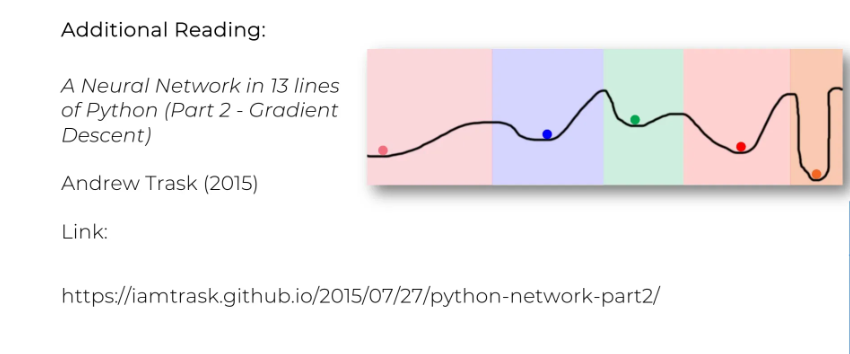
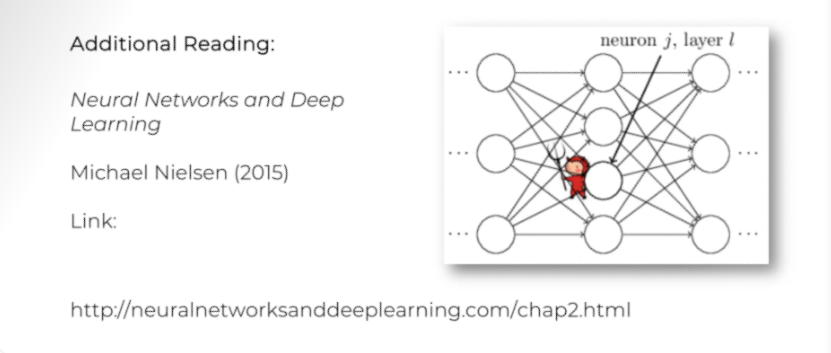
Another resource, a bit more detailed, is for those interested in the mathematics. If you want to understand why gradient descent works the way it does, what formulas drive it, and how it's calculated, check out this article, which is actually a book Neural Networks and Deep Learning.

Backpropagation

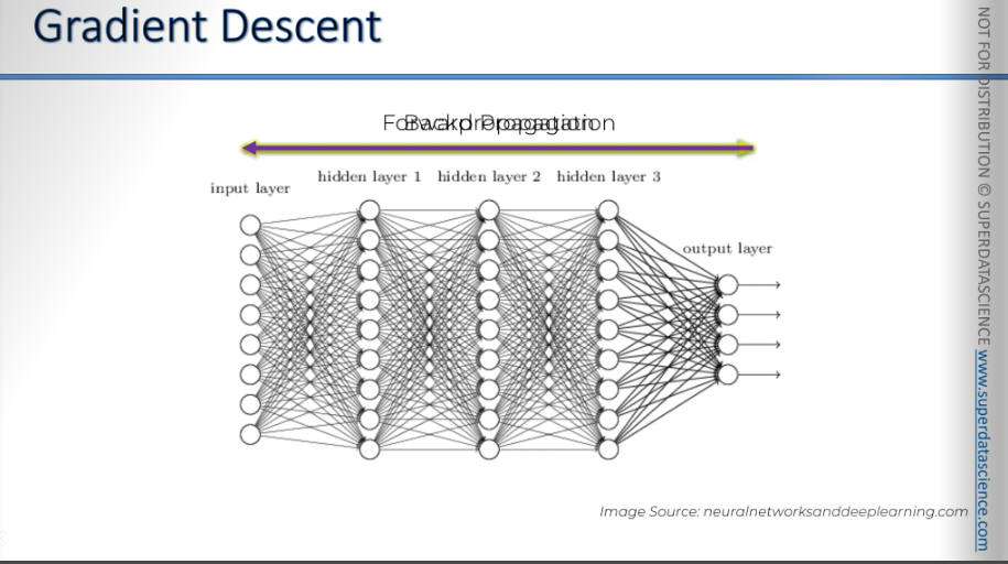
Alright, so we already know the basics of what happens in a neural network. We understand forward propagation, where information enters into the input layer and moves forward to get our predicted outputs, Y Hats. And then we compare those to the actual values that we have in our training set, and then we calculate the errors. Then the errors are back propagated through the network in the opposite direction. This process helps us train the network by adjusting the weights.

The key point to remember here is that backpropagation is an advanced algorithm based on complex mathematics. It allows us to adjust all the weights at the same time. Backpropagation adjusts all of the weights at the same time.

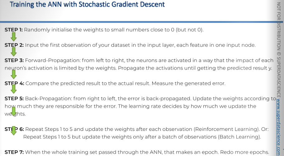
Step-by-step walkthrough of what happens during the training of a neural network:

1. Randomly initialize the weights to small numbers close to zero, but not exactly zero. Weights need a starting point, so they are set with random values near zero. Through forward propagation and backpropagation, these weights are adjusted until the error and the cost function are minimized.

2. Input the first observation of your data set into the first row of the input layer, with each feature as one input node. Essentially, take the columns and put them into the input nodes.

3. Forward propagation: Activate the neurons from left to right. The effect of each neuron's activation is controlled by the weights, which decide how important each neuron's activation is. Continue passing the activations until you get the predicted result, Y Hat. Move from left to right until you reach the end and get your Y Hat.

4. Compare the predicted result to the actual result and measure the generated error.

5. Perform backpropagation from right to left, updating the weights based on their contribution to the error. The learning rate determines how much we update the weights, and it's a parameter you can control in your neural network.

6. Step six involves repeating steps one to five and updating the weights after each observation. This process is known as reinforcement learning, and in our case, it was stochastic gradient descent. Alternatively, you can repeat steps one to five but update the weights only after a batch of observations, which is called batch learning. This can be done through full gradient descent, batch gradient descent, or mini-batch gradient descent.

7. And step seven, when all the data has passed through the artificial neural network, it completes one epoch. Repeat more epochs. Essentially, keep doing this process over and over, allowing your neural network to train and improve continuously, adjusting itself as you minimize the cost function.

Business problem description

ANN in python

Get code and dataset from: Machine Learning

Now we are going to build an artificial brain. We will actually create a deep neural network with neurons and fully-connected layers linking these neurons.

We will apply this to a business problem, as usual. The dataset we'll be working with resembles a real-world dataset, containing many observations and features. We will predict an outcome, which will be a binary variable. It's important to know that artificial neural networks can be used for both regression and classification. In this case, we will use it for classification.

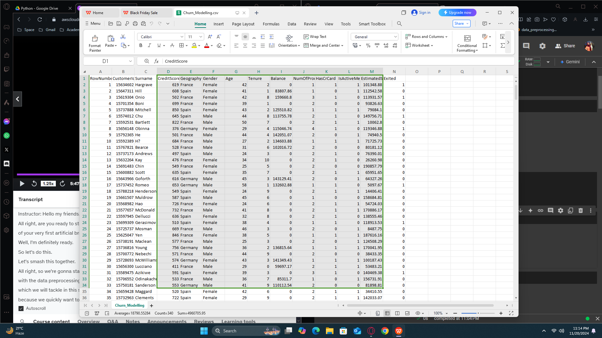
About the dataset: this time we have many features. This is the data set of a bank which collected some information about their customers.

• Customer ID

• Surname

• Credit score

• Geography (country the customer lives in)

• Gender

• Age

• Tenure (number of years they have been with the bank)

• Balance (amount of money in their account)

• Number of products used from the bank (e.g., credit card, checkbook, MasterCard, loan, home loan)

• Has credit card (1 if yes, 0 if no)

• Is active member (1 if active, 0 if not)

• Estimated salary (salary estimated by the bank)

• Exited (dependent variable: 1 if the customer left the bank, 0 if they stayed)

What happened in reality was that the bank observed all of its customers for about 6 months, let's say. Additionally, the bank collected all the other features too, to see the correlation between these features and whether the customer stays with the bank or leaves. Makes sense right? It is important to figure out why people are leaving cause a bank makes money from the customers. So, their goal is to keep as many customers as possible, so they created this dataset to understand why customers leave.

And mostly, once they managed to build a predictive model, model that was trained on this data set, they will be able to predict if any new customer leaves the bank. They will use this model for new customers. For any customer the model predicts will leave the bank, they will be ready to offer special deals to encourage them to stay. This approach aims to keep as many customers as possible from leaving the bank.

And why is this called churn modeling? Because customer churn refers t o the situation where some customers leave.

We have a lot to do! This will be a long implementation, but it is definitely worth it! Deep learning is one of the most powerful areas of machine learning. Alright, let's get started.

Part 1: Data pre-processing

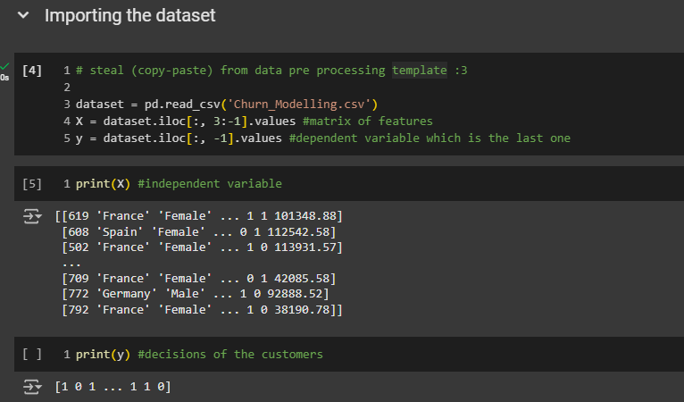
Look at here. The first three columns actually has no impact on figuring out whether the customer will leave or stay. Although our neural network will figure it out on its own but let;s just make the process easier by exclusing them. We will take the column from index 3 to -1, alr?

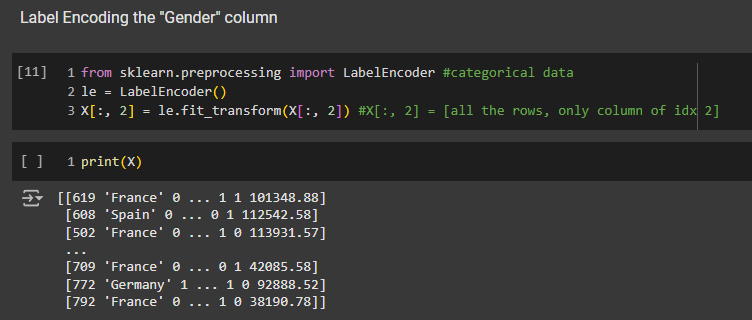
Lebel encoding to the gender column: 0 → female, 1 → male

This time, we need to use one-hot encoding because there is no order between France, Spain, and Germany. We can't just assign France as zero, Spain as one, and Germany as two. Hence, we have to use one-hot encoding. So, let's do that.

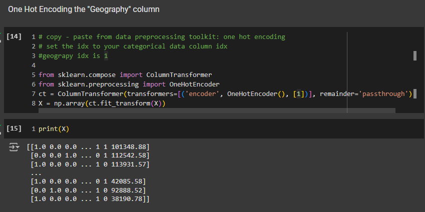
Remember, when we perform one-hot encoding, the dummy variables are moved to the first columns of the feature matrix. So, we have them right here in the first three columns, which is the initial set of dummy variables. France is encoded as 100, Spain as 001, and Germany as 010.

Splitting the dataset into the Training set and Test set: We don't need to print these four entities since we understand how they work. However, feel free to do so if you wish. You're free to make any modifications to your copy, of course.

Feature Scaling: Absolutely fundamental. Feature scaling is absolutely compulsory for deep learning. Whenever you build an artificial neural network, you must apply feature scaling to all features, even if they already have values like zero and one. It's crucial for deep learning, so we scale everything

Part 2: Building the ANN

Initializing the ANN

We will initialize the ANN as a sequence of layers. We have to create a variable which is nothing else but the ANN itself.

This artificial neural network variable will be created as an object of a specific class. This class is the sequential class, which lets us build an artificial neural network as a sequence of layers, instead of a computational graph. As you learned, an artificial neural network is a series of layers, starting with the input layer and followed by fully connected layers, ending with the final output layer.

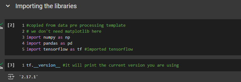
ann = tf.keras.models.Sequential()

The sequential class comes from the models module in the Keras library, which is now part of TensorFlow since version 2.0. We use tf to call TensorFlow, then the Keras library, and the models module, to access the sequential class. This creates the ANN variable, representing our artificial neural network as a sequence of layers.

Adding the input layer and the first hidden layer

There’s actually no rule for how many neurons we’ll need. You have to figure it out from your experience. For me, i tried it with 7 and different other numbers but all of them gave me pretty much same result so yah, feel free to explore and check with different values.

Also, in the intuition blog, you saw that the hidden layers of a fully connected neural network must use the rectifier activation function, which is what we need to specify here.

ann.add(tf.keras.layers.Dense(units = 6, activation = 'relu'))

# Add a dense (fully connected) layer to the Artificial Neural Network (ANN)
# units=6: number of neurons in this layer
# activation="relu": rectified linear unit activation function

Adding the second hidden layer

You can use this add method to add anything, and adding a second hidden layer is just like adding the first one. Of course, you can change the number of hidden neurons if you want, but having six neurons in the first hidden layer and another six in the second hidden layer works well. Again, feel free to experiment.

#add method can add any new layer. 

ann.add(tf.keras.layers.Dense(units=6, activation='relu'))

Adding the output layer

It contains what we want to predict.

• Since we have a binary variable, a binary outcome, you only need one neuron to encode these outcomes as either one or zero.

• For the output layer's activation function, use a sigmoid instead of a rectifier. A sigmoid function provides not just predictions but also the probability of a binary outcome being one. This means we'll know not only if a customer will leave the bank but also the likelihood of it happening, thanks to the sigmoid activation function. So, use the sigmoid activation function for the output layer.

ann.add(tf.keras.layers.Dense(units=1, activation='sigmoid'))

Part 3: Training the ANN

Compiling the ANN

# instance_name.method(optimizer, loss function, metrics[])
ann.compile(optimizer = 'adam' , loss = 'binary_crossentropy' , metrics = ['accuracy'])

For the optimizer, which one should you choose?

Remember, the best optimizers are those that can perform stochastic gradient descent. The one I recommend by default is the Adam Optimizer, which is a very efficient optimizer capable of performing stochastic gradient descent. Let me remind you what stochastic gradient descent does. It updates the weights to reduce the error between your predictions and the actual results. When we train the ann on the training set, we compare the predictions in each batch to the real results in that batch. The optimizer will update the weights using stochastic gradient descent. We will choose the Adam optimizer to hopefully reduce the loss in the next iteration.

When performing binary classification and predicting a binary outcome, always use the binary_crossentropy as the loss function. For non-binary, you gotta use categorical_crossentropy. Also, when doing non-binary classification the activation should be ‘soft max’ okay?

Training the ANN on the Training set

We're about to train the artificial neural network on the training set over 100 epochs. The method to train any machine learning model is always the same. It is the fit method.

If you don't want to spend too much time tuning this hyperparameter, I recommend choosing the default value of 32 for the batch size.

A neural network needs to be trained over a certain number of epochs to improve accuracy over time. We can simply use 100 epochs. You can use any number but don’t go below 100, as you neural network needs certain amounts of epochs to learn properly.

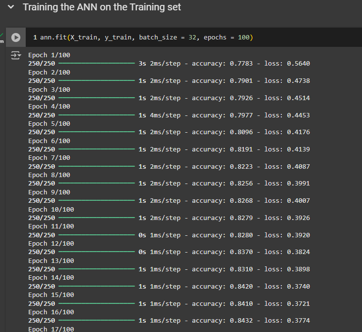
And we can see that it is actually increasing pretty fast. It is also converging, you pretty quickly. We converged at 0.86, about T the 20th Epic.

The final accuracy on the training set is about 0.86. We'll need to check the test set for comparison. That means you have 86 correct predictions out of 100 observations.

Part 4: Making the predictions and evaluating the model.

[I hope you did well with the homework on the colab file]

Predicting the Test set results

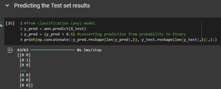
As we can see, the predictions are quite accurate. we don't have all the results displayed because we have a lot of observation.

However, the first customer actually stayed with the bank and was predicted to stay. However, the second customer left the bank but was predicted to stay. The third customer stayed with the bank and was predicted to stay as well. For the last three customers in the test set, they all stayed with the bank and were predicted to stay. So, the results look very good.

Making the Confusion Matrix

We achieve an accuracy of over 86%. That's impressive because it means that out of 100 customers, 86 were correctly predicted to either stay with or leave the bank.

We have

• 1,528 correct predictions that the customer stays with the bank

• 200 correct predictions that the customer leaves the bank

• 67 incorrect predictions that the customer leaves the bank

• 205 incorrect predictions that the customer stays with the bank

So anyway, that looks pretty good!

You completed a pretty advanced branch of machine learning. You should really be proud of your progress.

As soon as you feel ready for it, well, join me, in the next blog to learn convolution neural networks. And until then, enjoy machine learning!

ANN Quiz