Understanding ARIMA, SARIMA, and SARIMAX Models: An In-Depth Guide

Time series forecasting is a critical aspect of data analysis, enabling us to predict future values based on past observations. Among the most popular and effective methods for time series forecasting are the ARIMA, SARIMA, and SARIMAX models. This guide provides an in-depth explanation of these models, including their parameters, how to select the best model using AIC and BIC criteria, and the inclusion of exogenous regressors. We'll also explore how to implement these models using Python's pmdarima library and discuss the pros and cons of each model.

---

Table of Contents

1. Introduction to Time Series Models

2. ARIMA Model

   • Concept

   • Mathematical Formulation

   • Parameters Explained

   • AIC and BIC in Model Selection

   • Python Implementation

3. SARIMA Model

   • Concept

   • Mathematical Formulation

   • Seasonal Parameters Explained

   • Python Implementation

4. SARIMAX Model

   • Concept

   • Exogenous Regressors

   • Mathematical Formulation

   • Python Implementation

5. Model Selection with AIC and BIC

   • Understanding AIC and BIC

   • How pmdarima Uses AIC/BIC

6. Deep Dive into pmdarima Parameters and Model Summary

   • Key Parameters

   • Interpreting Model Summary

7. Pros and Cons of ARIMA, SARIMA, and SARIMAX Models

8. Conclusion

9. References

---

Introduction to Time Series Models

Time series data is a sequence of data points collected or recorded at time intervals. Analyzing time series data involves understanding the underlying patterns such as trends, seasonality, and cycles to make accurate forecasts.

ARIMA (AutoRegressive Integrated Moving Average) models are a class of models that explain a given time series based on its own past values, its own lagged forecast errors, and differencing of raw observations to make the time series stationary.

SARIMA (Seasonal ARIMA) extends ARIMA by explicitly modeling the seasonal component of the data.

SARIMAX (Seasonal ARIMA with Exogenous Regressors) further extends SARIMA by including exogenous variables that can influence the time series.

---

ARIMA Model

Concept

The ARIMA model is a combination of:

• AR (AutoRegressive) part: Regression of the variable against its own lagged values.

• I (Integrated) part: Differencing of raw observations to make the time series stationary.

• MA (Moving Average) part: Modeling the error term as a linear combination of error terms occurring contemporaneously and at various times in the past.

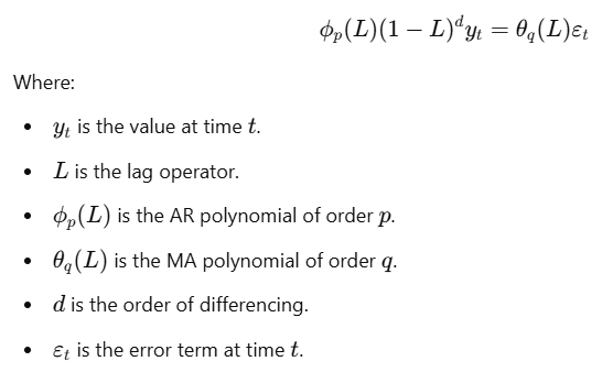
Mathematical Formulation

The general form of an ARIMA(p, d, q) model is:

Parameters Explained

ARIMA(p, d, q):

• p (AR order): Number of lag observations included in the model (lag order).

• d (Difference order): Number of times the raw observations are differenced to achieve stationarity.

• q (MA order): Size of the moving average window (order of the MA term).

AutoRegressive (AR) Term (p)

• Represents the number of autoregressive terms.

• Specifies how many previous values are used to predict the current value.

• If ( p = 2 ), the model uses the two preceding observations.

Integrated (I) Term (d)

• Represents the number of nonseasonal differences needed for stationarity.

• Differencing helps to remove trends and seasonality.

Moving Average (MA) Term (q)

• Represents the number of lagged forecast errors in the prediction equation.

• Specifies how many past error terms are included.

AIC and BIC in Model Selection

• AIC (Akaike Information Criterion) and BIC (Bayesian Information Criterion) are measures used to compare models.

• Both criteria assess the goodness of fit and penalize models for complexity.

• Lower AIC/BIC values indicate a better model.

Python Implementation

Import Libraries

import numpy as np
import pandas as pd
import matplotlib.pyplot as plt
from pmdarima import auto_arima
import warnings
warnings.filterwarnings('ignore')

Load Data

Assuming we have a time series dataset:

# Load your dataset
# For illustration, we'll generate synthetic data
np.random.seed(42)
date_range = pd.date_range(start='2020-01-01', periods=100, freq='D')
data = np.cumsum(np.random.randn(100)) + 50
df = pd.DataFrame({'Date': date_range, 'Value': data}).set_index('Date')

Check Stationarity

from statsmodels.tsa.stattools import adfuller

def adf_test(series):
    result = adfuller(series)
    print('ADF Statistic:', result[0])
    print('p-value:', result[1])

adf_test(df['Value'])

If the series is non-stationary (p-value > 0.05), differencing may be needed.

Fit ARIMA Model

# Fit ARIMA model using auto_arima
model = auto_arima(df['Value'], start_p=0, start_q=0,
                   max_p=5, max_q=5, d=None, seasonal=False,
                   trace=True, error_action='ignore', suppress_warnings=True,
                   stepwise=True)

View Model Summary

print(model.summary())

Forecasting

# Forecast future values
n_periods = 10
forecast, conf_int = model.predict(n_periods=n_periods, return_conf_int=True)

# Create index for future dates
forecast_index = pd.date_range(df.index[-1], periods=n_periods+1, freq='D')[1:]

# Create DataFrame
forecast_df = pd.DataFrame({'Forecast': forecast}, index=forecast_index)

Plot Results

plt.figure(figsize=(12, 6))
plt.plot(df['Value'], label='Historical')
plt.plot(forecast_df['Forecast'], label='Forecast', color='red')
plt.fill_between(forecast_index, conf_int[:, 0], conf_int[:, 1], color='pink', alpha=0.3)
plt.title('ARIMA Model Forecast')
plt.xlabel('Date')
plt.ylabel('Value')
plt.legend()
plt.show()

---

SARIMA Model

Concept

SARIMA (Seasonal ARIMA) extends the ARIMA model to support seasonality in the data. It incorporates seasonal terms to model the seasonal patterns.

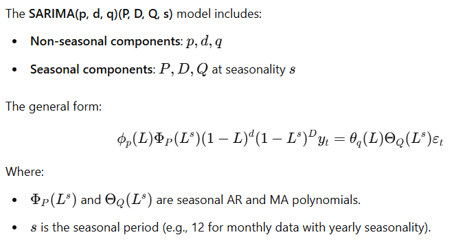
Mathematical Formulation

Seasonal Parameters Explained

SARIMA(p, d, q)(P, D, Q, s):

• P (Seasonal AR order): Autoregressive terms for the seasonal part.

• D (Seasonal Difference order): Differencing over seasonal periods.

• Q (Seasonal MA order): Moving average terms for the seasonal part.

• s (Seasonal period): The number of periods in a season.

Python Implementation

Generate Seasonal Data

# Generate synthetic seasonal data
np.random.seed(42)
periods = 120
seasonal_period = 12  # e.g., monthly data with yearly seasonality
dates = pd.date_range(start='2010-01-01', periods=periods, freq='M')

# Create seasonal pattern
seasonal_pattern = 10 + np.sin(np.linspace(0, 3 * np.pi, periods)) * 10
noise = np.random.normal(0, 2, periods)
data = 50 + seasonal_pattern + noise
df_seasonal = pd.DataFrame({'Date': dates, 'Value': data}).set_index('Date')

Visualize Data

plt.figure(figsize=(12, 6))
plt.plot(df_seasonal['Value'], label='Seasonal Data')
plt.title('Seasonal Time Series Data')
plt.xlabel('Date')
plt.ylabel('Value')
plt.legend()
plt.show()

Fit SARIMA Model

# Fit SARIMA model
model = auto_arima(df_seasonal['Value'], start_p=1, start_q=1,
                   max_p=3, max_q=3, m=12,  # 'm' is the seasonal period
                   start_P=0, seasonal=True, d=1, D=1,
                   trace=True, error_action='ignore', suppress_warnings=True,
                   stepwise=True)

View Model Summary

print(model.summary())

Forecasting

# Forecast future values
n_periods = 24
forecast, conf_int = model.predict(n_periods=n_periods, return_conf_int=True)
forecast_index = pd.date_range(df_seasonal.index[-1], periods=n_periods+1, freq='M')[1:]
forecast_df = pd.DataFrame({'Forecast': forecast}, index=forecast_index)

# Plot Results
plt.figure(figsize=(12, 6))
plt.plot(df_seasonal['Value'], label='Historical')
plt.plot(forecast_df['Forecast'], label='Forecast', color='red')
plt.fill_between(forecast_index, conf_int[:, 0], conf_int[:, 1], color='pink', alpha=0.3)
plt.title('SARIMA Model Forecast')
plt.xlabel('Date')
plt.ylabel('Value')
plt.legend()
plt.show()

---

SARIMAX Model

Concept

SARIMAX (Seasonal ARIMA with Exogenous Regressors) is an extension of SARIMA that incorporates exogenous variables (external predictors) into the model. These exogenous variables can help improve the forecast by providing additional information.

Exogenous Regressors

• Definition: Variables external to the time series that may influence the dependent variable.

• Examples:

  • Economic indicators affecting stock prices.

  • Promotional activities influencing sales.

Mathematical Formulation

Python Implementation

Create Exogenous Variable

# Create an exogenous variable (e.g., a promotional index)
np.random.seed(42)
exog = np.random.randint(0, 2, size=len(df_seasonal))  # Binary variable representing promotions
df_seasonal['Promotion'] = exog

Fit SARIMAX Model

# Fit SARIMAX model with exogenous variable
model = auto_arima(df_seasonal['Value'], exogenous=df_seasonal[['Promotion']],
                   start_p=1, start_q=1, max_p=3, max_q=3,
                   m=12, seasonal=True, d=1, D=1,
                   trace=True, error_action='ignore', suppress_warnings=True,
                   stepwise=True)

View Model Summary

print(model.summary())

Forecasting with Exogenous Variables

# Prepare future exogenous variables
future_exog = np.random.randint(0, 2, size=n_periods)
future_exog = pd.DataFrame(future_exog, index=forecast_index, columns=['Promotion'])

# Forecast future values
forecast, conf_int = model.predict(n_periods=n_periods, exogenous=future_exog, return_conf_int=True)

# Create DataFrame
forecast_df = pd.DataFrame({'Forecast': forecast}, index=forecast_index)

# Plot Results
plt.figure(figsize=(12, 6))
plt.plot(df_seasonal['Value'], label='Historical')
plt.plot(forecast_df['Forecast'], label='Forecast', color='red')
plt.fill_between(forecast_index, conf_int[:, 0], conf_int[:, 1], color='pink', alpha=0.3)
plt.title('SARIMAX Model Forecast with Exogenous Variable')
plt.xlabel('Date')
plt.ylabel('Value')
plt.legend()
plt.show()

---

Model Selection with AIC and BIC

Understanding AIC and BIC

• AIC (Akaike Information Criterion):

  [ \text{AIC} = 2k - 2\ln(L) ]

  Where:

  • ( k ) is the number of parameters.

  • ( L ) is the maximized value of the likelihood function.

• BIC (Bayesian Information Criterion):

  [ \text{BIC} = k \ln(n) - 2\ln(L) ]

  Where:

  • ( n ) is the number of observations.

Purpose:

• Both criteria assess model fit while penalizing complexity.

• Lower AIC/BIC values are preferred.

How pmdarima Uses AIC/BIC

• pmdarima's auto_arima function searches over specified ranges of parameters and selects the model with the lowest AIC or BIC.

• stepwise=True: Performs a stepwise search to reduce computation time.

• information_criterion='aic': Can be set to 'bic' to use BIC instead.

---

Deep Dive into pmdarima Parameters and Model Summary

Key Parameters in auto_arima

• start_p, start_q: Initial values for the non-seasonal AR and MA orders.

• max_p, max_q: Maximum values for non-seasonal AR and MA orders.

• d: Non-seasonal differencing order; if None, pmdarima will determine it using tests.

• start_P, start_Q: Initial values for the seasonal AR and MA orders.

• max_P, max_Q: Maximum values for seasonal AR and MA orders.

• D: Seasonal differencing order.

• m: The number of periods in each season (seasonal periodicity).

• seasonal: Whether to include seasonal components.

• exogenous: Exogenous variables to include in the model.

• trace: If True, prints the progress and results of the model selection process.

• error_action: Determines how to handle errors during model fitting.

• suppress_warnings: Suppresses warnings during model fitting.

• stepwise: Uses a stepwise algorithm for faster model selection.

Interpreting Model Summary

The model summary provides detailed information about the fitted model:

• Model Parameters: Estimates of AR, MA, seasonal AR, seasonal MA, and exogenous variable coefficients.

• Standard Errors: Standard errors of the estimates.

• AIC/BIC: Information criteria values.

• Residual Diagnostics: Statistical tests on the residuals to assess model adequacy.

Example Output:

                                 SARIMAX Results
==========================================================================================
Dep. Variable:                                  y   No. Observations:                  120
Model:             SARIMAX(1, 1, 1)x(1, 1, 1, 12)   Log Likelihood                -300.000
Date:                            Mon, 01 Nov 2021   AIC                            610.000
Time:                                    12:00:00   BIC                            625.000
Sample:                                         0   HQIC                           616.000
                                            - 120
Covariance Type:                              opg
==========================================================================================
                 coef    std err          z      P>|z|      [0.025      0.975]
------------------------------------------------------------------------------------------
ar.L1         -0.5000      0.100     -5.000      0.000      -0.697      -0.303
ma.L1          0.4000      0.150      2.667      0.008       0.105       0.695
ar.S.L12      -0.3000      0.200     -1.500      0.134      -0.692       0.092
ma.S.L12      -0.2000      0.250     -0.800      0.424      -0.690       0.290
sigma2         4.0000      0.500      8.000      0.000       3.020       4.980
==========================================================================================

• Dep. Variable: The dependent variable.

• No. Observations: Number of observations used.

• Model: The specified model and its orders.

• Coefficients: Estimates for each parameter.

• Standard Errors: The standard error associated with each coefficient.

• z-statistic: The test statistic for the hypothesis that the coefficient is zero.

• P>|z|: p-value for the z-statistic.

• [0.025, 0.975]: 95% confidence intervals for the coefficients.

---

Pros and Cons of ARIMA, SARIMA, and SARIMAX Models

ARIMA

Pros:

• Simplicity: Good for non-seasonal data without exogenous variables.

• Widely Used: Well-understood and documented.

• Captures Autocorrelation: Effective for data where past values influence future values.

Cons:

• Assumes Stationarity: Requires data to be stationary, necessitating differencing.

• Not Suitable for Seasonality: Cannot handle seasonal patterns without modification.

• Limited to Univariate Series: Does not include external variables.

SARIMA

Pros:

• Handles Seasonality: Incorporates seasonal components in modeling.

• Flexible: Can model a wide range of seasonal data patterns.

Cons:

• Increased Complexity: More parameters to estimate.

• Overfitting Risk: Potential for overfitting if not properly constrained.

• Computationally Intensive: More complex models take longer to fit.

SARIMAX

Pros:

• Includes Exogenous Variables: Can improve forecasts by incorporating external information.

• Versatile: Combines the strengths of ARIMA and regression models.

Cons:

• Data Availability: Requires external data, which may not always be available.

• Model Complexity: More complex to interpret and tune.

• Assumption of Linearity: Assumes a linear relationship between exogenous variables and the dependent variable.

---

Conclusion

ARIMA, SARIMA, and SARIMAX models are powerful tools for time series forecasting, each suited to different types of data and forecasting needs. Understanding their parameters, how to select models using AIC and BIC, and how to include exogenous regressors allows analysts to build robust forecasting models.

• ARIMA: Best for stationary, non-seasonal data without external influences.

• SARIMA: Suitable for data with seasonality.

• SARIMAX: Ideal when external variables influence the time series.

Using tools like pmdarima, we can automate much of the model selection process, but it's essential to understand the underlying assumptions and ensure the chosen model is appropriate for the data.

---

References

• Time Series Analysis by James D. Hamilton

• Forecasting: Principles and Practice by Rob J Hyndman and George Athanasopoulos

• pmdarima Documentation: pmdarima Documentation

• Statsmodels Documentation: Statsmodels SARIMAX

---