Welcome to Part 8.2 - Deep Learning! Deep Learning is the most exciting and powerful branch of Machine Learning.

If you're new to this blog, I strongly advise you to read the previous blogs because this one is quite advanced. Thank you!

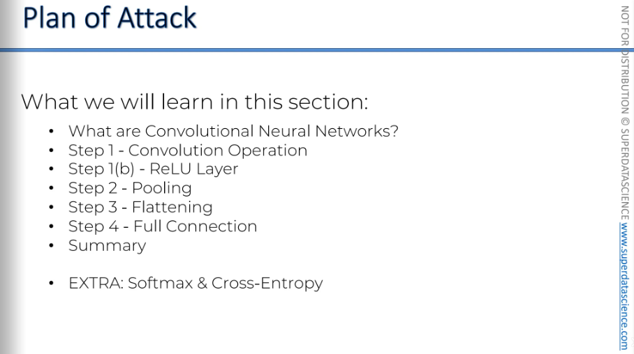
Plan of attack

This is our plan of attack. We will be covering this in our blog.

CNN intuition

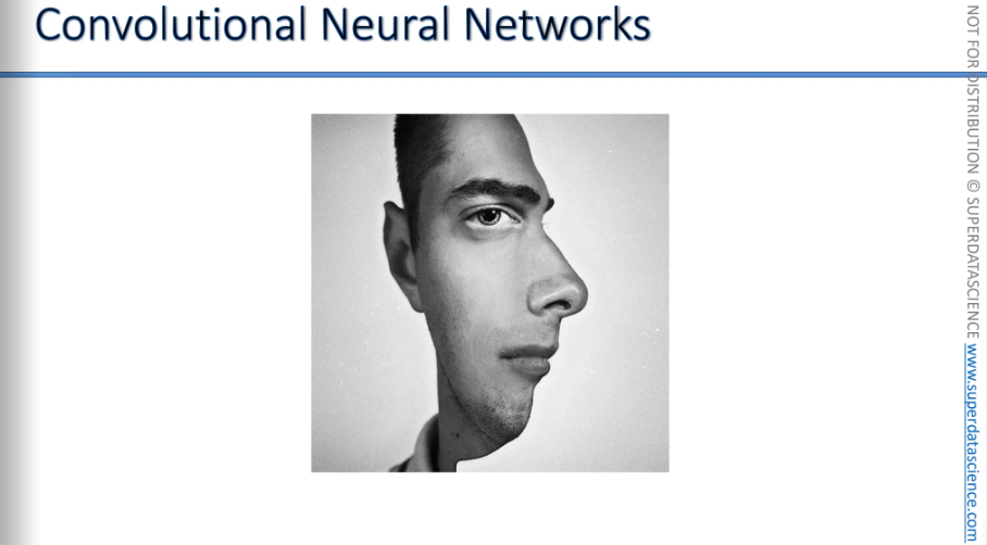
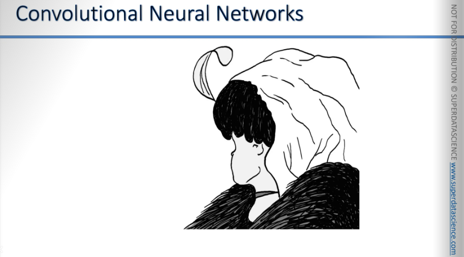
What do you see when you look at this image? Do you see a person looking at you? Or do you see a person looking to the right?

You can tell that your brain is having a hard time deciding. This shows that when our brain looks at things, it searches for features. Based on the features it detects and processes, it categorizes things in specific ways.

So let's take a look at another image. This is a very famous picture. But what do you see here?

Some people will say they see a young lady wearing a dress, looking away.
Some people will say they see an old lady wearing a scarf on her head, looking down.

As you can see, it's two images in one. Depending on which features your brain notices, it will switch between classifying the image as one or the other.

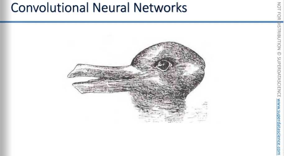
The oldest recorded illusion of this type in print is this one: the duck or the rabbit. So, is it a duck, or is it a rabbit?

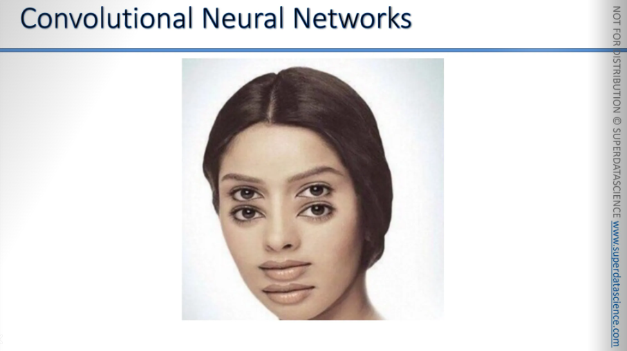
So, what do you see? Do you feel a bit dazzled, like your brain is trying to figure out what it is? It's as if your mind is jumping between her eyes, moving up and down.

This is a classic example of when certain features could represent different things, but your brain can't decide because both options seem possible.

These examples show us how the brain works. It processes certain features in an image or in what you see in real life and classifies them accordingly.

You've probably experienced moments when you quickly glance over your shoulder and see something. You might think it's a ball, but it turns out to be a cat, or you think it's a car, but it's actually a shadow. This happens because you don't have enough time to process those features or there aren't enough features to classify things accurately.

Do you see how the brain processes images? When understanding images, our neural network does something very similar.

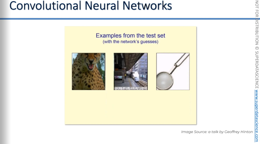
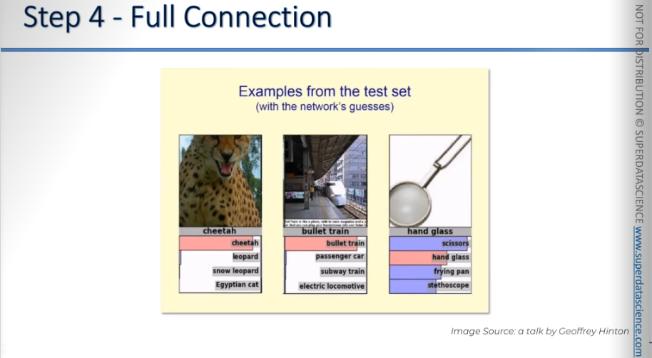
Here's an experiment done on computers using convolutional neural networks. This slide is from a talk by Geoffrey Hinton, showing an experiment he did several years ago with some convolutional neural networks he trained. The neural network correctly recognized the first two images: a cheetah and a bullet train. But it said the third image was scissors, while it was actually a magnifying glass. The third image isn't very clear either, therefore the neural network was confused.

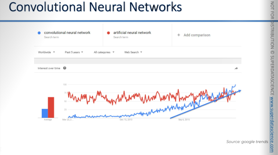
Here, you can see that convolutional neural networks are becoming more popular than artificial neural networks. They are growing fast and will continue to do so because this is a crucial area. This is where important things happen, like self-driving cars recognizing people and stop signs on the road. It's also how Facebook can tag images or people in photos.

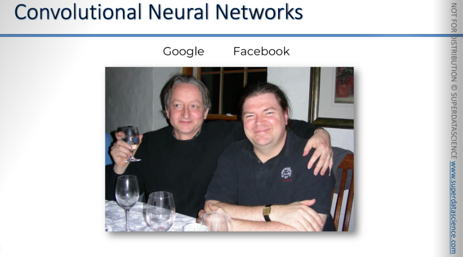
Speaking of Facebook, if Geoffrey Hinton is the godfather of artificial neural networks and deep learning, then Yann LeCun is the grandfather of convolutional neural networks.

Yann LeCun was a student of Geoffrey Hinton, who is now leading deep learning efforts at Google. Yann LeCun is the director of Facebook's artificial intelligence research and also a professor at NYU.

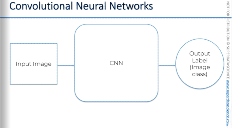
How CNN works? It’s very simple. You have an input, an input image. The input image goes through CNN and you get an output label, which CNN classifies as an Image.

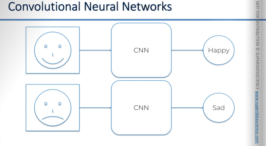
Let’s say, a neural network has been trained up to recognize facial expression. Now if you give it an image of a person or, even a drawing like this - smiley, it will tell you the person is happy and the vice versa.

As you can see it is already very powerful in terms of so many different applications.

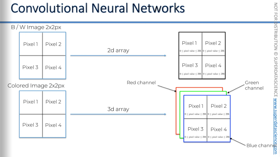
How can a neural network recognize these features? It all begins at a very basic level. Imagine you have two images.

One is a black-and-white image with two-by-two pixels, and the other is a colored image with two-by-two pixels. Neural networks use the fact that the black-and-white image is a two-dimensional array. What we see visually is just a representation, but in computer terms, it's a two-dimensional array where each pixel has a value between 0 and 255.( This represents eight bits of information, as 2^8 equals 256, so the values range from 0 - 255, showing the intensity of the color, specifically white).

A value of 0 is a completely black pixel
255 is a completely white pixel

And the values in between represent different shades of gray. With this information, computers can process the image.

Every image has a digital representation made up of ones and zeros that form a number from 0 to 255 for each pixel. This is what the computer processes, not the colors themselves, but the binary data. This is the foundation of how it all works.

And in colored image, it’s actually a 3D array. You have a blue layer, a green layer, and a red layer, which stand for RGB. Each of these colors has its own intensity. Essentially, a pixel has three values assigned to it, each ranging from 0 to 255. By combining these three values, you can determine the exact color of the pixel. Computers work with this data, and that's the foundation of how it all operates.

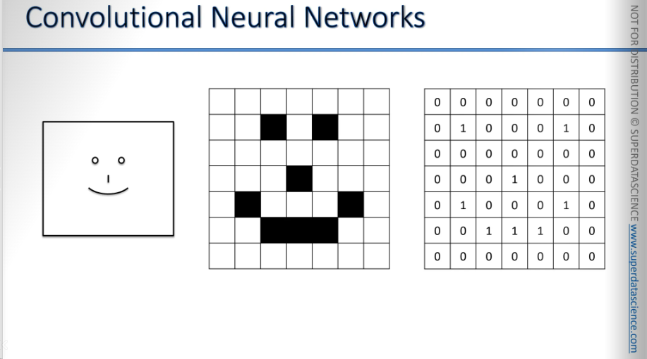
Now, let’s loot at a very trivial example of a smiling face. Just for simplicity’s sake, let’s not take all the 255 values. Let’s just take 0 → white and 1 → black and start our example okay?

We will be looking at very simple structure but at the same time all of these concepts can be translated back to the 0-255 rage of values.

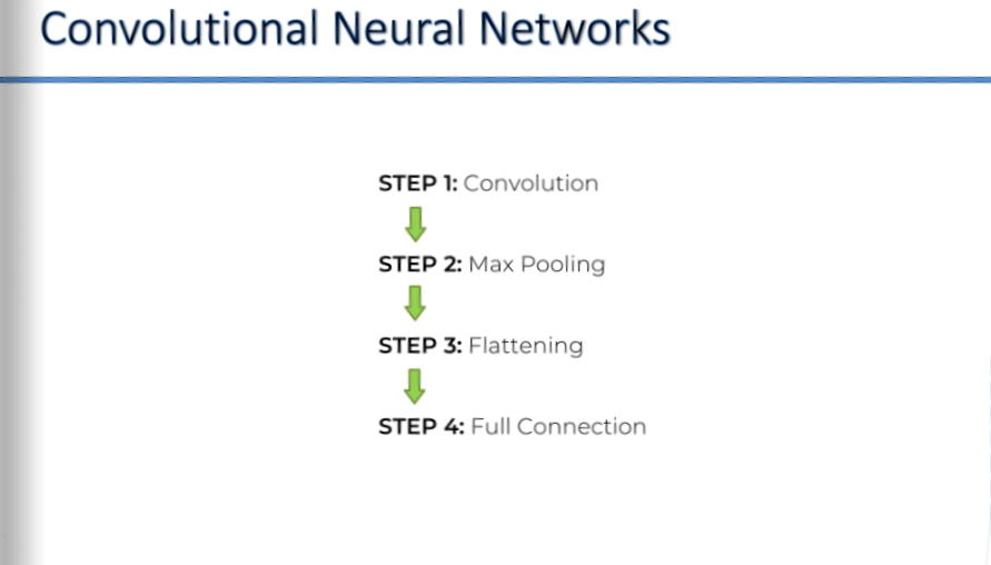
These are the steps we will be going through.

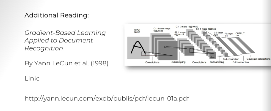
The additional reading you might want to explore is Yann LeCun's original paper that led to the development of convolutional neural networks. It's called Gradient-Based Learning Applied to Document Recognition.

Convolution Operation

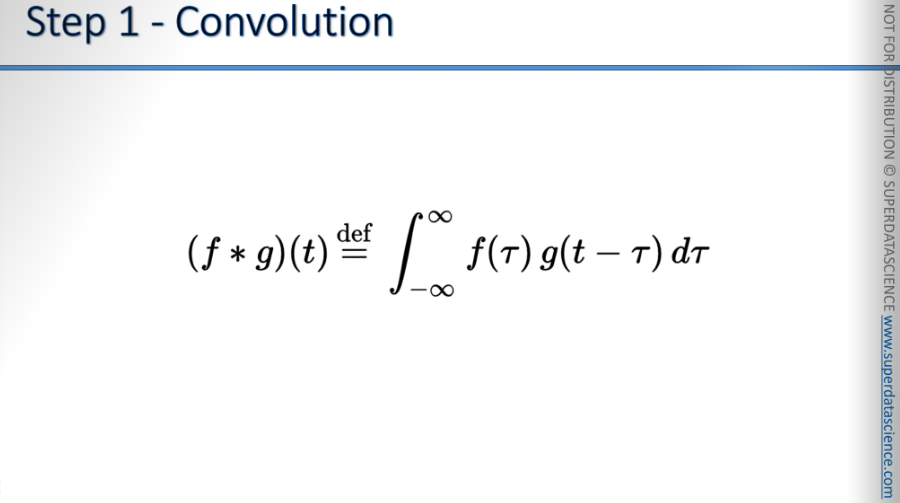
This is the convolution function. A convolution is basically a combined integration of two functions.

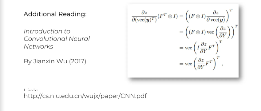
if you'd like to get into the math behind the convolution neural networks, a great additional read is Introduction to Convolution Neural Networks by Jianxin Wu, who is a professor at the Nanjing University in China. In the URL, if you remove the last two parts and go to /WJX, you'll reach his homepage. There, you can find more tutorials and materials that haven't been published as papers but are used in his tutorials. You might find these useful.

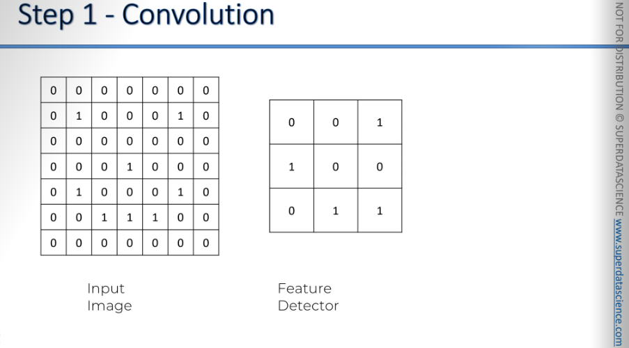
So, Here on the left we've got an input image of just 1's and 0's to simplify things. Can you see there’s a smiley face there?

Anyways, we have a feature detector of 3×3 (could be 7×7, 5×5, not necessarily always 3×3). Also, there are other names for feature detector too, i.e., kernel, filter etc.

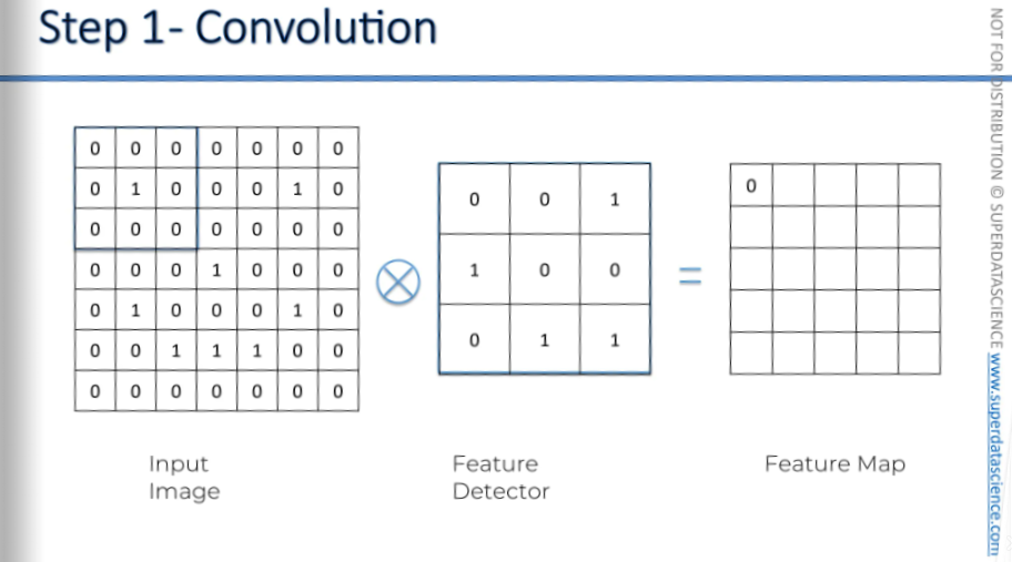
A convolution operation is signified by an X in a circle. What is actually happening here is- you take this feature detector and you put it on your image.So you cover the top left corner, the 9 pixels in the top left corner, and multiply each value by the corresponding value. For example, the top left value is multiplied by the top left value, position 1,1 by position 1,1, position 0,1 by 0,1, 0,2 by 0,2, and so on.

This is called element-wise multiplication of these matrices. Then, you add up the results. In this case, nothing matches, so it's always either 0 by 0 or 0 by 1. The result is 0.

Here you can see one of them matched up, therefor we got an 1 here.

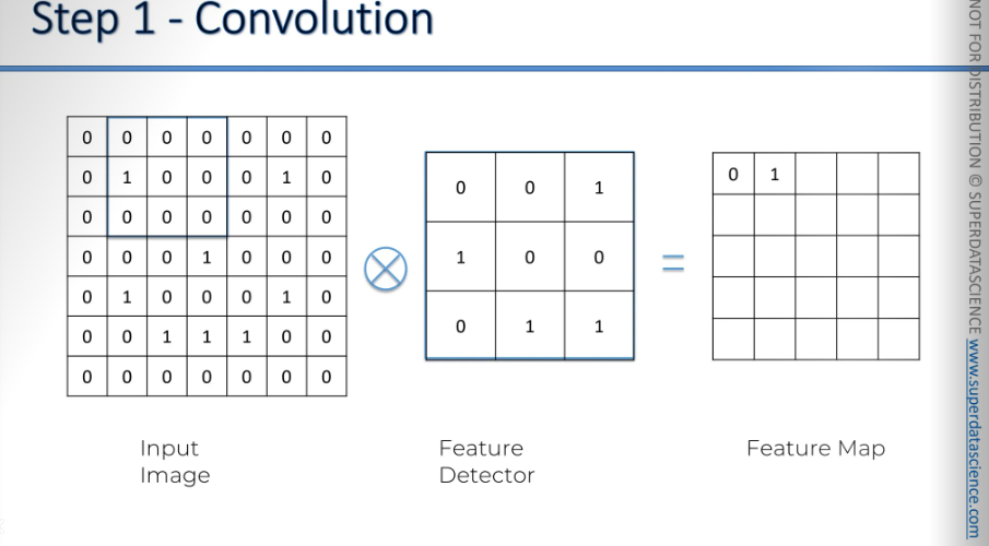
Then we move to the next one and the step at which we're moving this whole filter is called the stride.

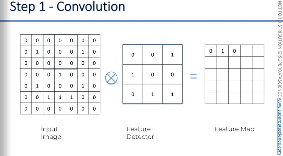
And do on, we are done. So, what have we created, right? Couple of important things here.

The image on the right is called a feature map. Also has many names, i.e., convolved feature, activation map etc.
we've reduced the size of the image. This is important cause it makes the process easier.
Are we losing information? Yes, we lose some because the resulting matrix has fewer values. However, the feature detector's purpose is to identify key features of the image.

We don't examine every pixel; we focus on features like the nose, hats, feathers, or the black marks under a cheetah's eyes to tell it apart from a leopard, or the shape of a train. We eliminate what is unnecessary and focus only on the important features. These features are what matter to us. That is exactly what the feature map does.

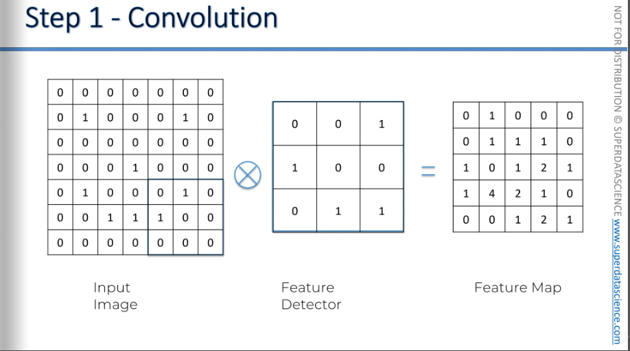
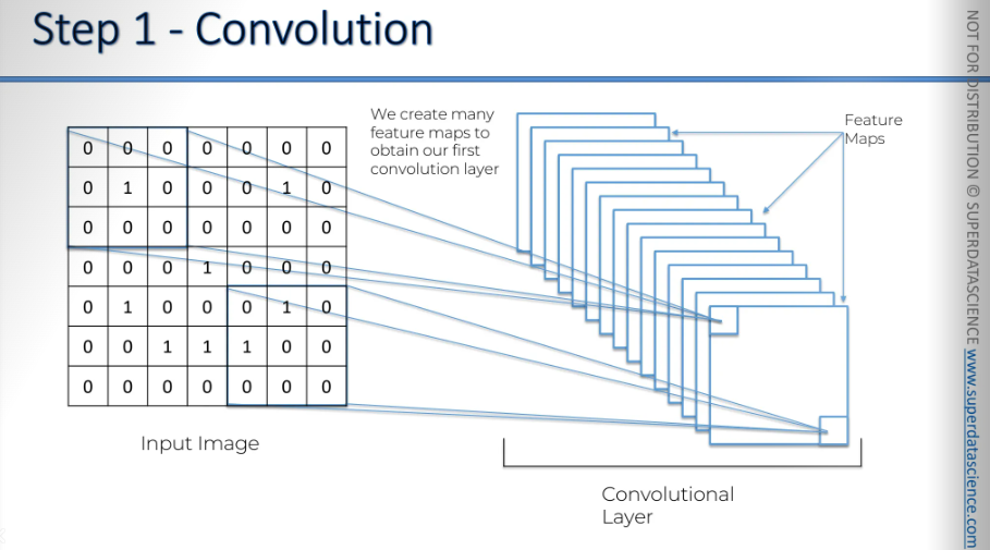
So now, moving on, on the left we have our input image, and on the right we created a feature map. The front one is the one we just made.

But why are there so many of them?

We create multiple feature maps because we use different filters. This helps us preserve a lot of information. Instead of just one feature map, we search for specific features. The network, through training, decides which features are important for certain categories and looks for them, using different filters.

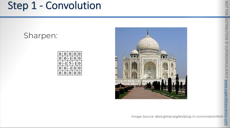
Let's look at a couple of examples. Using a tool from gimp.org, similar to Paint, you can adjust images. Their documentation includes useful examples. For instance, with a picture of the Taj Mahal, you can choose filters to apply. By downloading the program and uploading a photo, you can start a convolution matrix and apply filters.

If we apply this filter with 5 in the middle and -1 around it, you can see it sharpens the image. The 5 is the main pixel, and the -1 values reduce the surrounding pixels.

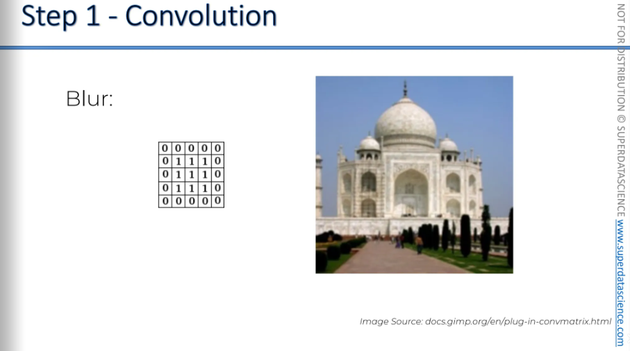
Then Blur. It gives equal importance to all surrounding pixels, combining them to create a blur.

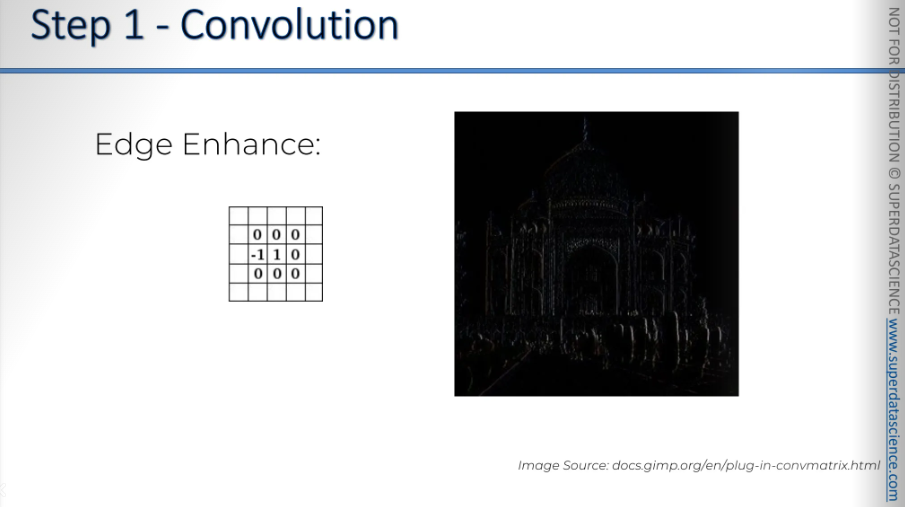
Edge Enhance. Here, you use -1 and 1 with 0's. You remove pixels around the main one, keeping it at -1, which enhances edges. This method is a bit tricky to grasp.

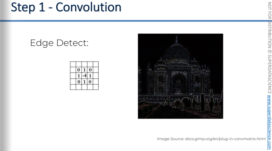
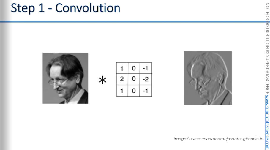
Edge Detect: You start by reducing the strength of the middle pixel. Then, you look for the 1's around it and increase their strength. This process highlights the edges, giving you an edge texture.

Emboss is another example. The key is that it's asymmetrical, and you can see the image becomes asymmetrical too. It gives the impression that the image is standing out towards you. This effect happens when you have negative values on one side and positive values on the other.

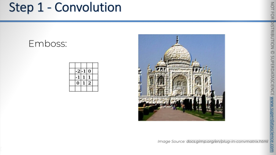
Edge Detect is probably the most important one for our type of work.

In terms of understanding, computers will decide for themselves. Their neural network will determine what is important and what is not. And that's the beauty of neural networks: they can process many things and understand which features are important without needing an explanation. The main purpose of a convolution is to find features in your image using the feature detector and place them into a feature map.

ReLU Layer

ReLU is rectified linear units and this is an additional step. It’s not a separate, It's step 1 B basically.

Here we have our input image and convolution layer, which we've discussed. We will apply ReLU on it now.

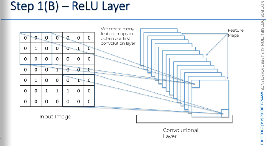
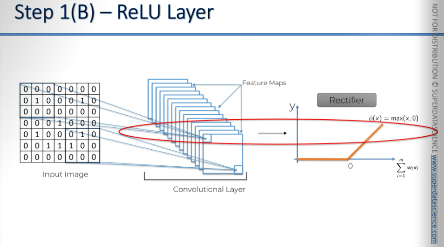
The reason we're applying the rectifier is to increase non-linearity in our image or network, specifically in our convolutional neural network. The rectifier acts as a filter or function that disrupts linearity.

We want to increase non-linearity in our network because images are very non-linear. This is especially true when recognizing different objects next to each other or against various backgrounds. Images have many non-linear parts, and the change between nearby pixels is often non-linear. This happens because of borders, different colors, and various elements in images.

However, when we use mathematical operations like convolution to detect features and create feature maps, we might end up with something linear. So, we need to break up the linearity.

Here is an original image.

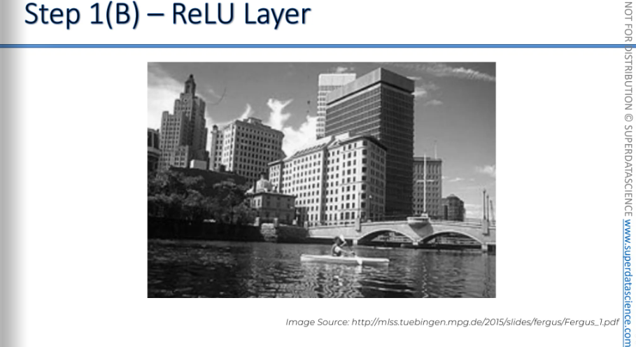
When we apply a feature detector to this image, we get a result like this. Here, black represents negative values, and white represents positive values.

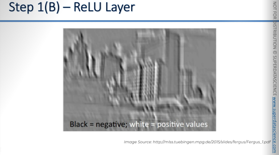
A rectified linear unit function removes all the black areas. Anything below zero becomes zero.

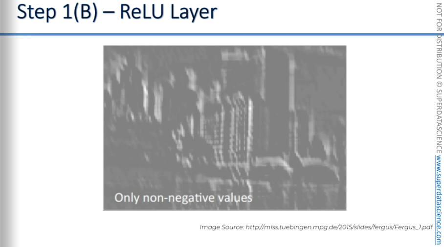
It's quite difficult to clearly see the benefit in terms of breaking up linearity. I'm sorry I can't explain it fully in writing. Ultimately, this is a very mathematical concept, and we would need to delve into a lot of math to truly understand what is happening.

If you'd like to learn more, there's a good paper. As always, there's always a paper.

This paper is by C.-C. Jay Kuo from the University of California, titled Understanding Convolutional Neural Networks With A Mathematical Model.

In the paper, he answers two questions, but you should focus on the first one: why a non-linear activation function is essential at the filter output of all intermediate layers. This explains the concept in more detail, both intuitively and mathematically. It's an interesting paper where you can find more information on this topic.

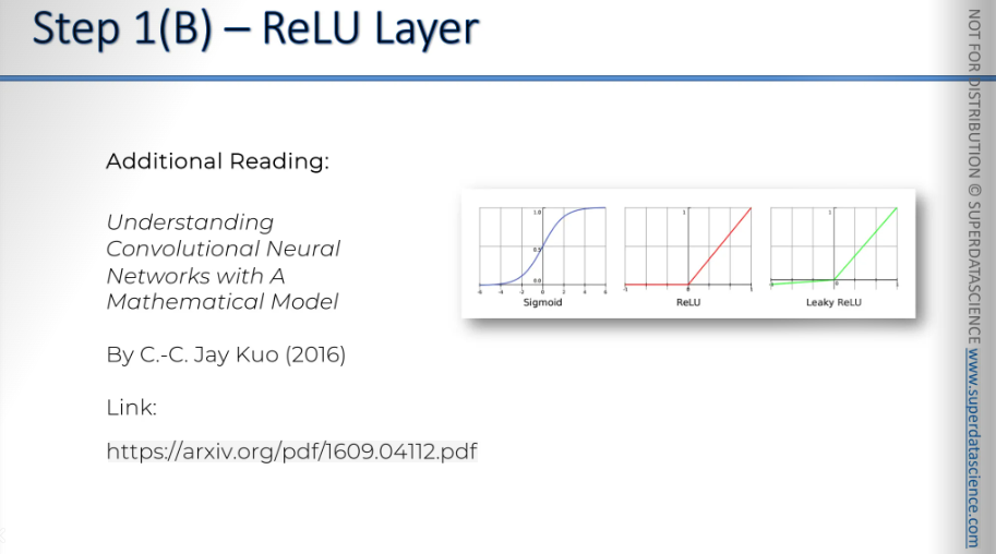
If you really want to dive in and explore some interesting things, there's another paper you can check out.

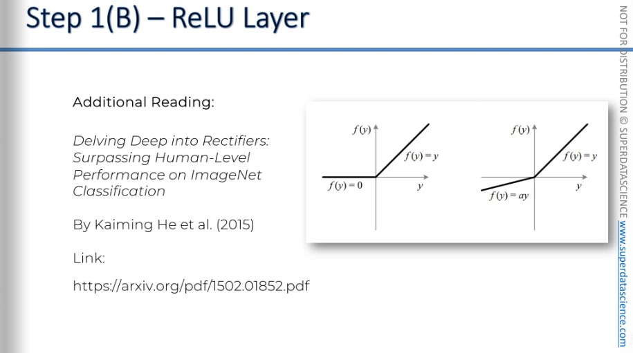
It's called Delving Deep into Rectifiers: Surpassing Human-Level Performance on ImageNet Classification.

Here, the authors, Kaiming He and others from Microsoft Research, propose a different type of rectified linear unit function. They introduce the parametric rectified linear unit function, shown on the right. They argue that it delivers better results without sacrificing performance. It's an interesting read.

Pooling

What is pooling and why do we need it?

Let's take a look at these images.

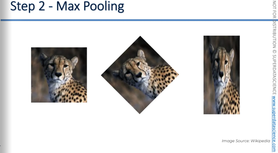
In these three images, we have a cheetah. In fact, it's the exact same cheetah. In the first image, the cheetah is positioned correctly and is looking straight at you. In the second image, it's slightly rotated, and in the third image, it's a bit squashed.

We want our neural network to recognize this cheetah.

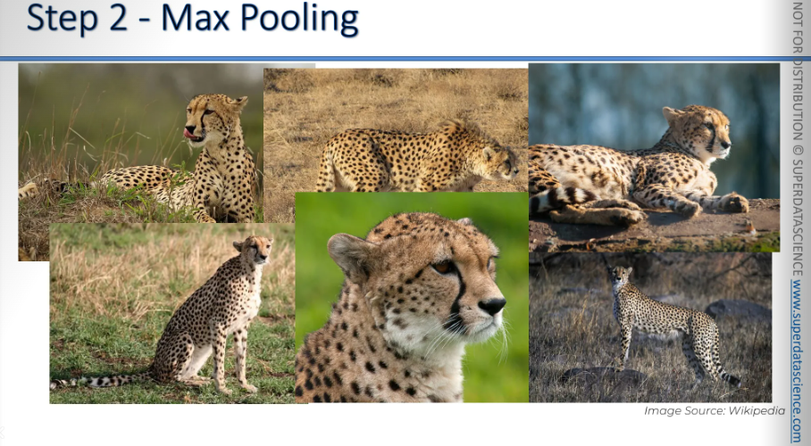
We want our neural network to recognize all of these cheetahs as cheetahs. They're all slightly different. The texture varies a little, and the lighting is different. There are many small differences.

So far, we have come to know that neural network looks for features from what it recognizes. Now, to give more flexibility, we will provide our neural network, a property called super invariance, means our neural network doesn’t care where are the features allocated.

It doesn't have to worry if the features are slightly tilted, if they have a different texture, if they are closer together, or if they are further apart relative to each other. Even if the feature itself is a bit distorted, our neural network needs some flexibility to still recognize that feature.

And that is what pooling is all about.

Here we have our feature map (convolution layer) on the left. Then we applied max pooling on it.

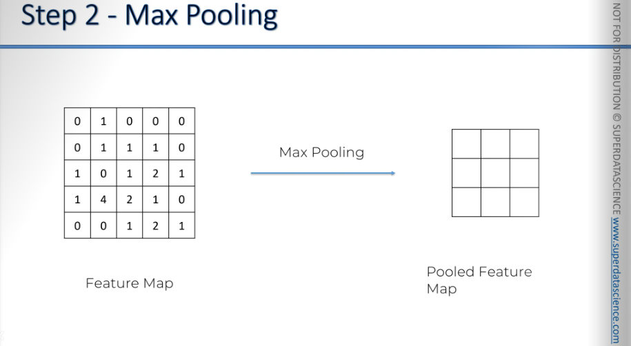
We take a box of 2x2 pixels like that (It doesn't have to be 2x2; you can choose any size for the box).Place it in the top left corner, find the maximum value in that box, and record only that value, ignoring the other three.

So, in your box, you have four values. You keep only one, the maximum, which is 1 in this case.

Then you move your box to the right by a stride and redo the process.

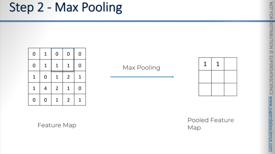
Here, as you can see it’s overlapping - but it really does not matter. You just keep repeating the process.

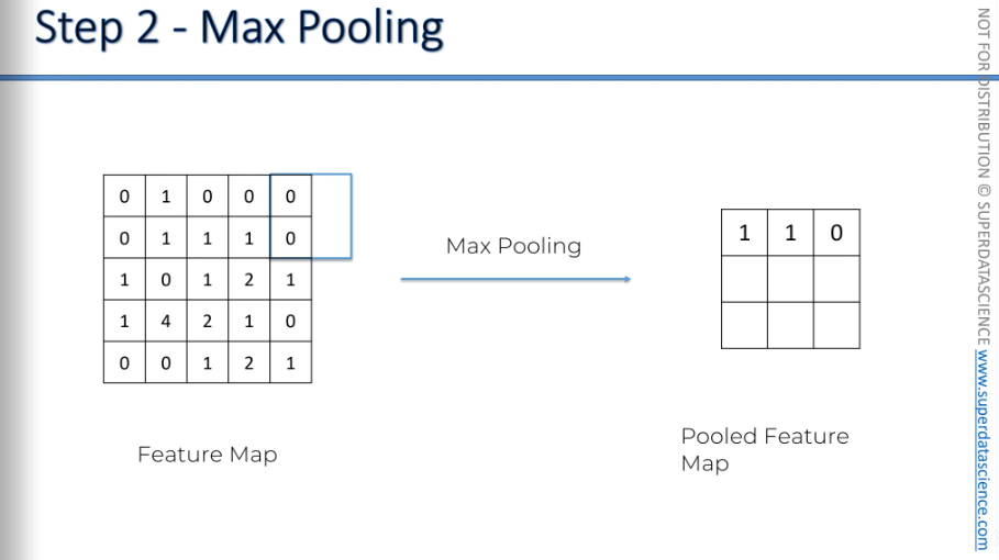
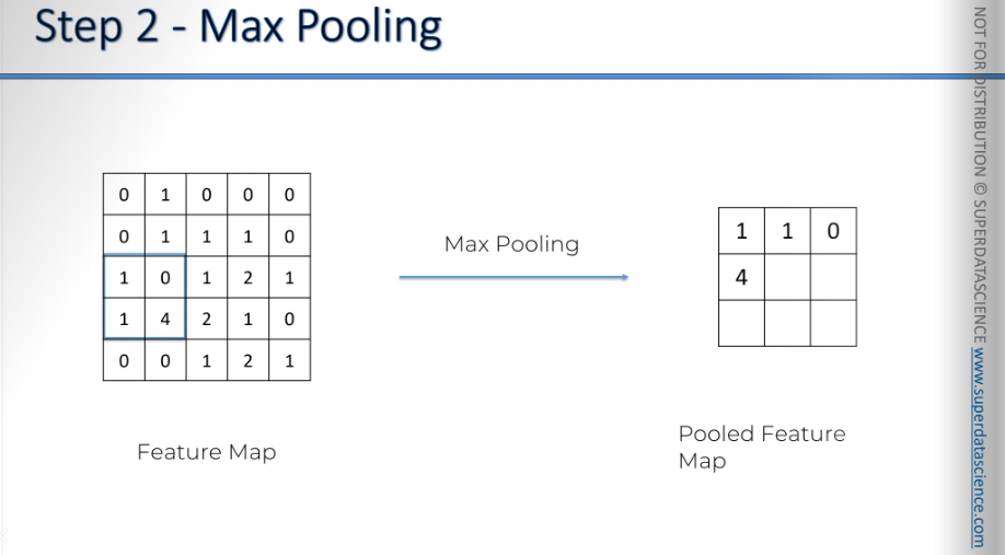
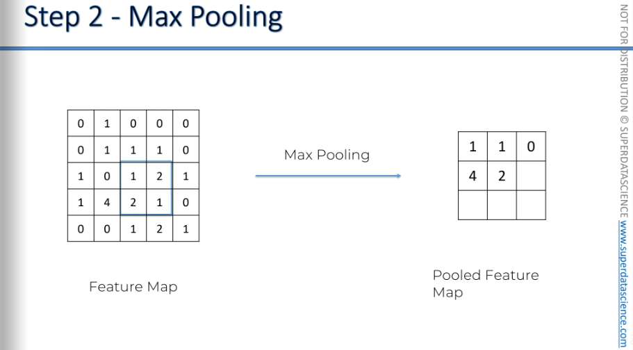
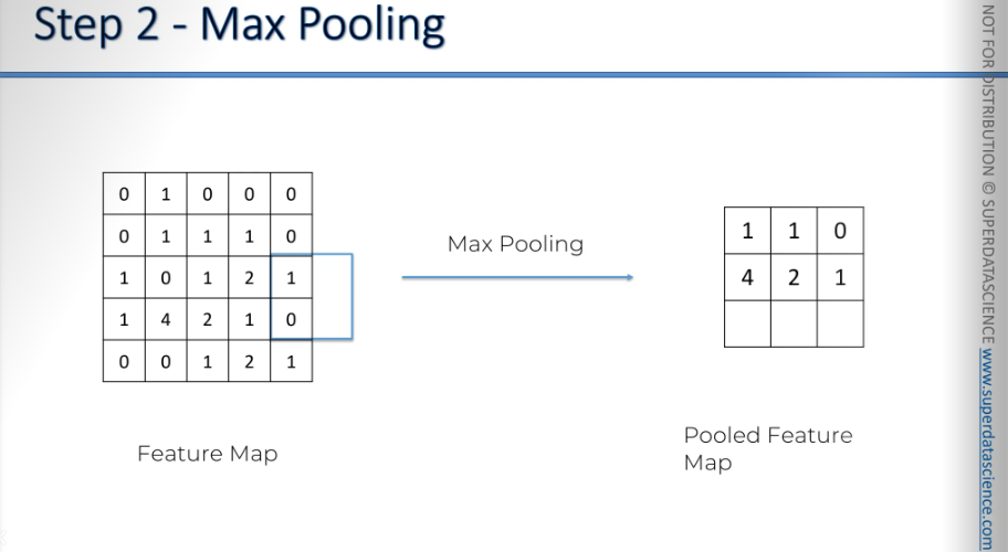
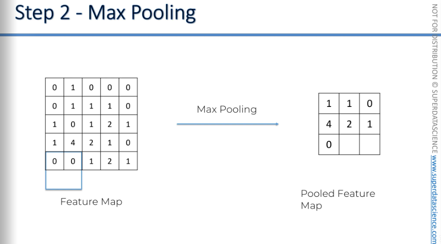
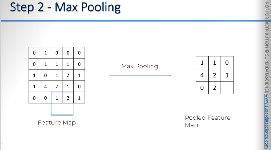
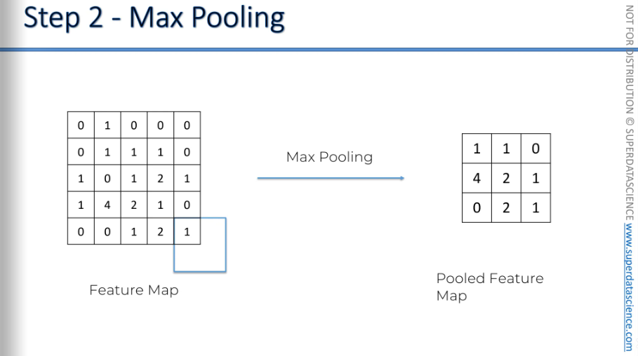
We can still keep the features, right? We know the biggest numbers show the features because we understand how the convolution layer works. The largest numbers in your feature map indicate where you found the closest match to a feature. By pooling these features, we remove 75% of the information that isn't part of the feature and isn't important. We're ignoring three out of four pixels, so we're only keeping 25%.

Another important thing is, we are preventing overfitting. As we are only keeping the relevant ones, our model will never be overfitted by information.

Even as a human, we don’t keep in mind all the information we see. We keep only the features which are necessary. Well, same thing for neural networks.

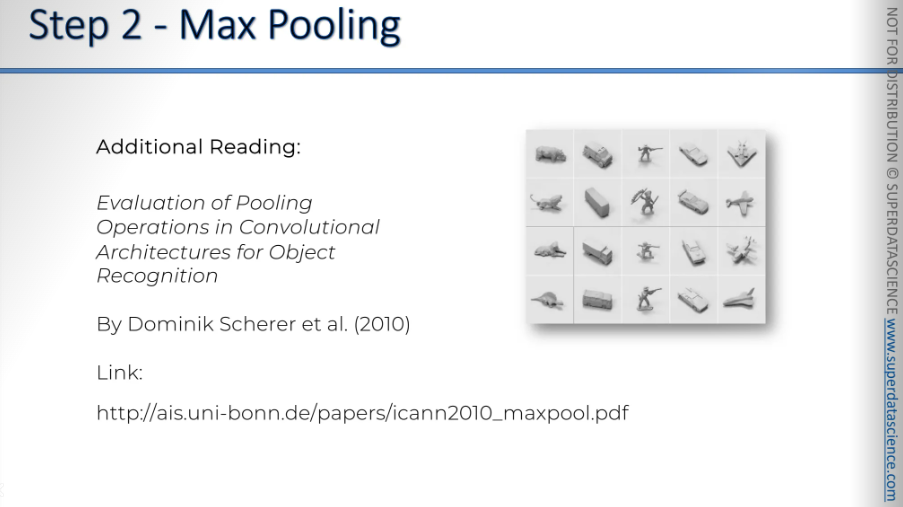
By the way, here's lots of different types of pooling and you know why, I'd like to introduce you to this lovely research paper called Evaluation of Pooling Operations in Convolution Architectures for Object Recognition by Dominic Sharer from University of Bon.

Now, it’s a recap:

Input image → convolution operation → convolution layer → pooling layer →

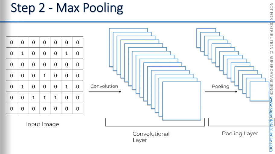
As we can see, even after having 25% of our information - our information was preserved. This is the main fact.

Click here

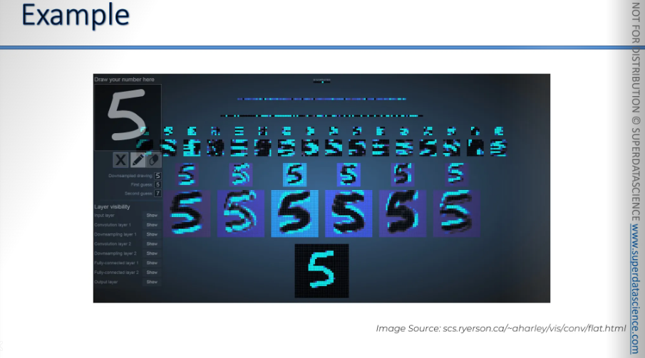
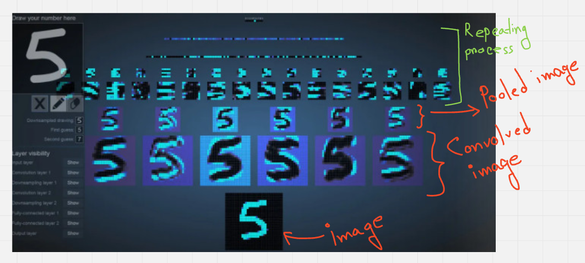
Flattening

This is a very simple step.

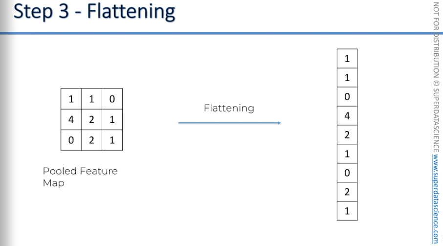
Okay so what are we going to do with this pooled feature map? We are going to flatten it into a column. Just take the numbers row by row and put them into this one long column.

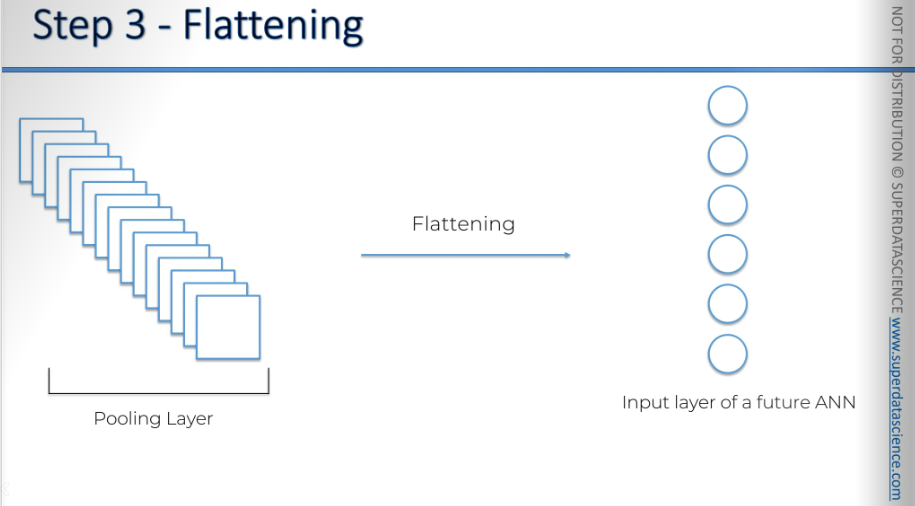
This is what it looks like when you have multiple pooling layers with many pooled feature maps, and then you flatten them.

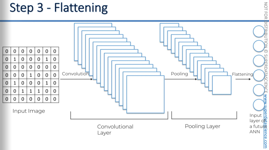
This is the flowchart.

Full Connection

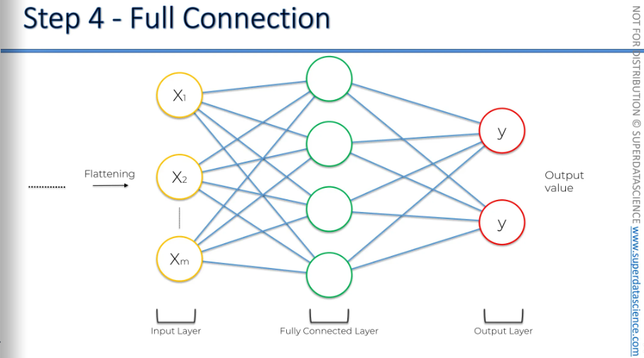
In this step, we're adding a complete artificial neural network to our convolutional neural network.

So, to everything we've done so far—convolution, pooling, and flattening—we're now adding a complete artificial neural network at the end. How intense is that?

Here, we have the input layer, a fully connected layer, and an output layer.

In artificial neural networks, what we used to call hidden layers are now referred to as fully connected layers. In artificial neural networks, hidden layers don't always have to be fully connected. However, in convolutional neural networks, we use fully connected layers, which is why they are generally called fully connected layers.

The main purpose of the artificial neural network is to combine our features into more attributes that predict the classes even better.

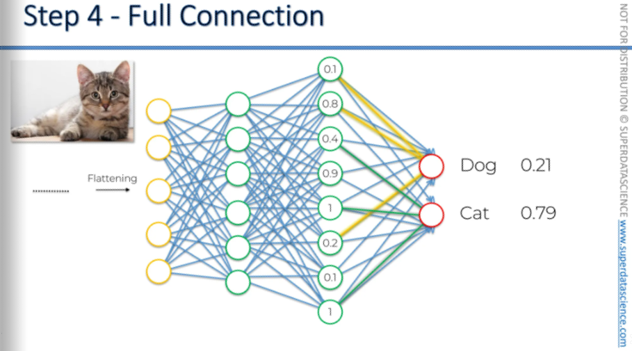
Here, we have a clearer artificial neural network with five inputs. The first hidden layer has six neurons. The second fully connected layer has eight neurons, and there are two outputs: one for dog and one for cat.

Alright, so we have done all the groundworks, the convolution, the pooling, the flattening - now all the information will go through this artificial neural network.

The yellow arrow shows the information moving from the beginning, starting when the image is processed, then convolved, pooled, flattened, and finally through the artificial neural network. All four steps. Then a prediction is made, and for instance, 80% that it's a dog, but it turns out to be a cat. And then an error is calculated. It's called a loss function. And we use a cross entropy function for that. Then the error is calculated, then it's back propagated through the network, and some things are adjusted in the network to help optimize the performance, such as:

The weights in the artificial neural network parts, the synopsis.
The feature detectors—what if we're looking for the wrong features? What if it doesn't work because the features are incorrect?

The feature detectors are adjusted, the weights are adjusted, and this whole process repeats. That's how our network is optimized.

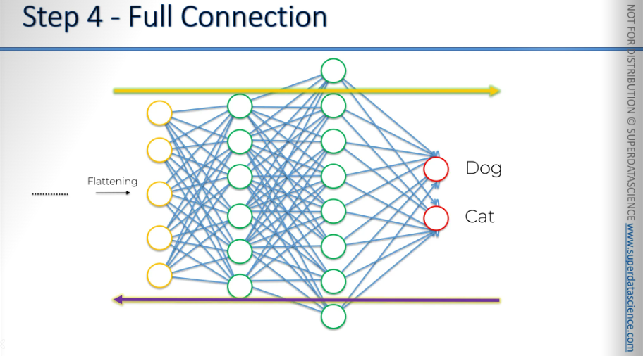
Let's start with the top neuron first.

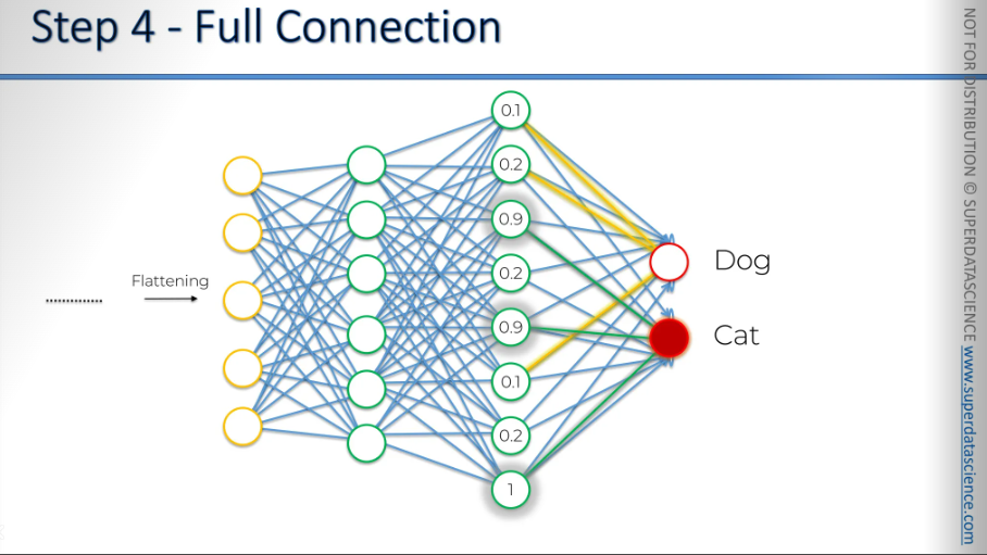
We'll begin with the dog. First, we need to understand what weights to assign to all the synapses that connect to the dog. This helps us determine which of the previous neurons are important for identifying the dog. Let's imagine we have some specific numbers in our previous fully connected layer or in the final fully connected layer.

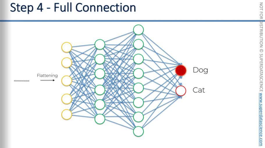
These numbers can be anything. They don't have to be specific, but for the sake of argument, we'll focus on numbers between zero and one. A value of one means the neuron is very confident it found a certain feature, while zero means the neuron didn't find the feature it was looking for. In the end, these neurons are just identifying features in an image.

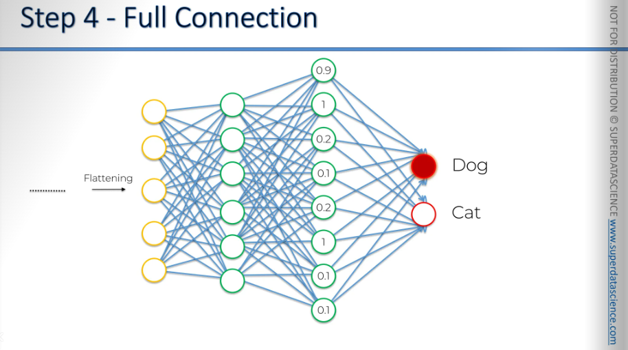
So a 1 which has been passed, and this is important has been passed to both the dog and the cat at the same time to both the output neurons.

So, when we say "one," it means this neuron is very active. It's quickly spotting a feature, like an eyebrow. For simplicity, let's say it's finding an eyebrow and sending this info to both the dog and cat neurons, saying, "I see an eyebrow." It's up to the dog and cat neurons to understand this.

In this situation, which neurons are active? These three neurons are active: the eyebrow, and let's say the nose, saying, "I see a big nose and floppy ears." They send this to both the dog and cat neurons.

Then, we realize this is a dog. The dog neuron knows it's a dog because we compare it to the picture or its label, confirming it's a dog. So, the dog neuron thinks, "Aha, I should be triggered here. These neurons are telling both me and the cat that it's actually a dog."

After many tries, if this keeps happening, the dog will learn that these neurons really activate when the feature is part of a dog.

On the other hand, the cat neuron will realize it's not a cat. It notices the feature is active, saying it sees floppy ears, but it's not a cat. This tells the cat neuron to ignore this signal. The more this happens, the more the cat neuron will ignore the floppy ears signal. Through many repetitions, if this happens a lot, the cat neuron will learn to disregard it. This is just one example, but if it happens often, maybe at a level of 1, or 0.8, or 0.9, sometimes it might not activate. But generally, if this neuron lights up often when it's a dog, the dog neuron will start to value this signal more. That's how we identify it.

We're going to say that these three neurons, through this repeated process with many samples and many epochs, learn over time. A sample is a part of your dataset, and an epoch is when you go through your entire dataset repeatedly. Through many iterations, the dog neuron learns that the eyebrow neuron, the big nose neuron, and the floppy ear neuron all help a lot in identifying a dog.

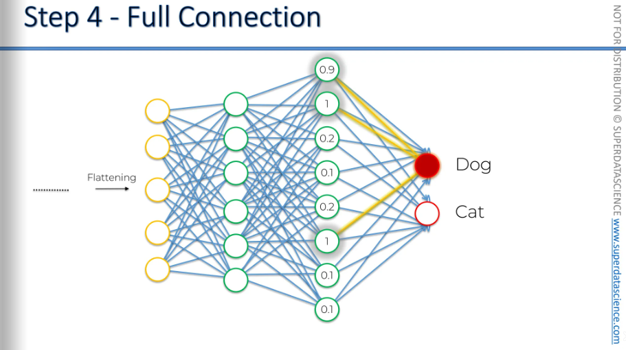
We are going to remmeber the Now let's focus on the cat neuron. We've already figured out the dog neurons. So, what is the cat neuron listening to? When it really is a cat, these three neurons, with values like 0.9, 0.9, and one, send signals to both the dog and cat neurons. It's important to remember that this signal goes to both. It tells the dog and the cat the same thing, but it's up to them to decide whether to use this information.

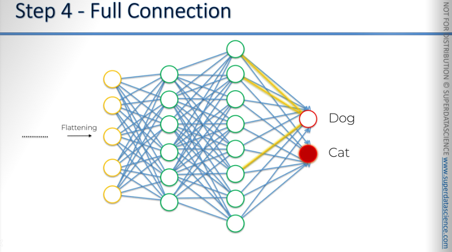
Imagine a photo of a cat. Both the dog and cat neurons can see it's a cat. The dog might notice the whiskers, pointy ears, and small size, or maybe the unique shape of cat eyes, which aren't circles but more like lines. These cat eyes aren't helping me predict anything. Every time these neurons activate, the prediction isn't right for me. But for the cat, it's different. When these neurons activate, it usually matches what the cat expects. So the cat decides to pay more attention to these signals. When they activate, the cat often gets a correct prediction, so it listens to them more. Some neurons don't activate even when it's a cat, so the cat ignores them. But when the cat eyes activate, it usually means it's a cat, so the cat learns to focus on those signals. Basically, the cat listens to these three neurons and ignores the other five. This is how the final neurons learn which signals to pay attention to in the fully connected layer.

That's how they understand. Basically, this is how features move through the network and reach the output. Even though features like floppy ears or whiskers might not mean much on their own, they are important for identifying a specific class. This is how the network learns.

During back propagation, we also adjust the feature detectors. If a feature doesn't help the output, it will likely be ignored over time. This happens through many iterations. Eventually, a useless feature is replaced by a useful one. In the final layer of neurons, you'll have many features or combinations that truly represent dogs and cats. Once your network is trained, this is how it works.

So, let's say we pass an image of a dog; the values are then propagated.

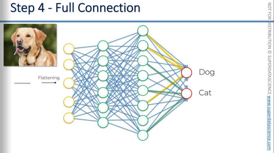
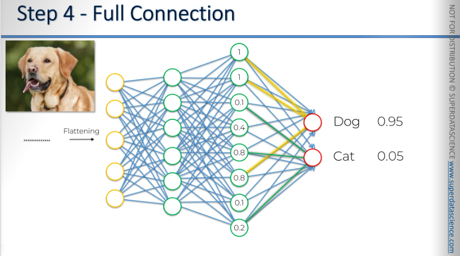
If they're a network, we get certain values. This time, the dog and cat neurons don't know if it's a dog or a cat because they don't have the image here. They have no idea what it is. But they have learned to pay attention to what's shown. The dog neuron checks three specific neurons, and the cat neuron checks another three. The dog neuron checks neurons 1, 2, and 3 and thinks, 'These values are high, so it's probably a dog.' The cat neuron checks its three and thinks, 'One value is high, but the others are low, so my probability is 0.05.' That's how you get your prediction.

The same thing happens when you pass an image of a cat. The probability might not be as high as before, but you can still see that it's a cat with 79% certainty. Therefore, the neural network will decide that it's a cat.

And that's how you get images like this:

You have a cheetah, and the network classifies it as a cheetah with high probability. Some probabilities are low, but they still exist because there's a small chance. Other neurons consider their inputs and might think, 'Oh, maybe it's actually a leopard.'

In another example, the network might predict a bullet train with high probability.

Scissors might be the top guess, but hand glass was a close second, followed by stethoscope. The scissors neuron paid attention to its inputs and got the most votes, but the hand glass also had a strong result.

So, that's how the full connection works and how everything comes together.

Summery

Let’s have a quick summery of all the things we have completed so far!

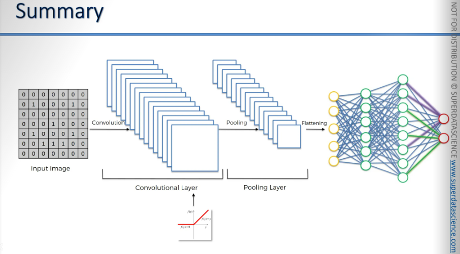
First of all, we started with an input image to which we applied multiple different feature detectors or, filters to create the feature maps and this is our convolutional layer. Then we applied ReLU (Refined Linear Unit) to remove linearities from the convoluted image. This increases non-linearity in our image. Then we applied pooling in every feature map and created a pooled feature map. The pooling does a lot of good things to us but the main fact is - it makes sure that our image has special invariance. It means, flexibility in picking up the features does not matter if it’s tilted, twsit3ed or even bit different from the ideal one. Another important thing it does is it gets rid of irrelevant features significantly, allowing us not to overfit our data but at the same time preserves main main features of our input image. Then we flatten all the pooled images into one column of vector. Then we input this into an artificial neural network. Afterward, the final step is the fully connected layer which performs the voting towards the classes that we’re after, then trained through forward propagation - backpropagation process, lots of iterations and epochs. And in the end, we have a very well defined neural network, where the weights are trained, feature detectors are trained plus adjusted in the, you know, the gradient descent process which allows us to get the best feature maps. Finally we get a convolution neural network which can recognize images and classify them.

Now you should be totally comfortable with this concept and ready to proceed to the practical applications.

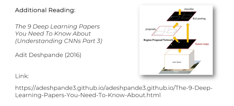
If you'd like to do some additional reading, there's a great blog by Adit Deshpande from 2016 called The 9 Deep Learning Papers You Need to Know About (Understanding CNNs Part 3)

This blog provides a brief overview of 9 different CNNs created by experts like Yann LeCun and others, which you can explore further. You'll encounter many new concepts that might be unfamiliar, but keep this blog and these nine papers in mind. Even if you're not ready to dive into them now, after the practical tutorials or some additional training in Deep Learning, you can refer back to these works. By examining other people's neural networks and how they structured their convolutional nets, you'll gain valuable insights into best practices and understand why certain design choices were made. This knowledge will assist you in developing your own neural network architectures.

Softmax and Cross-Entropy

This is an additional reading. I thought I’d be better for you know know about this as you are already going through CNN, so why not little bit extra?

Alright, in our main part we built a convolution network which, at the end 0.95 predicted that the given image is a fog and 5% probability that it’s a cat. This is after the training has been conducted.

My question is - how can 0.95 and 0.05 adds up to 1? Because, as far as we know, these two final neurons are not connected with each other. So, how do they know what the value of the other one is, and how do they know to add their values up to 1?

The thing is - they wouldn't in the classic version of artificial neural network.The only reason they do is because we use a special function called the softmax function to help us.

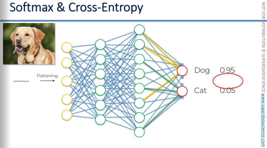
Normally, the cat and the dog will have any kind of real values which doesn’t have to be add up to 1. But when we apply the SoftMax function on them, their values will be ranged between 0-1, which would also make them add up to 1.

It makes sense to introduce the SoftMax function (normalized exponential function) into convolutional neural networks because it would be strange if you had possible classes of a dog and a cat, and the probability for the dog class was 80% while the probability for the cat class was 45%, right?

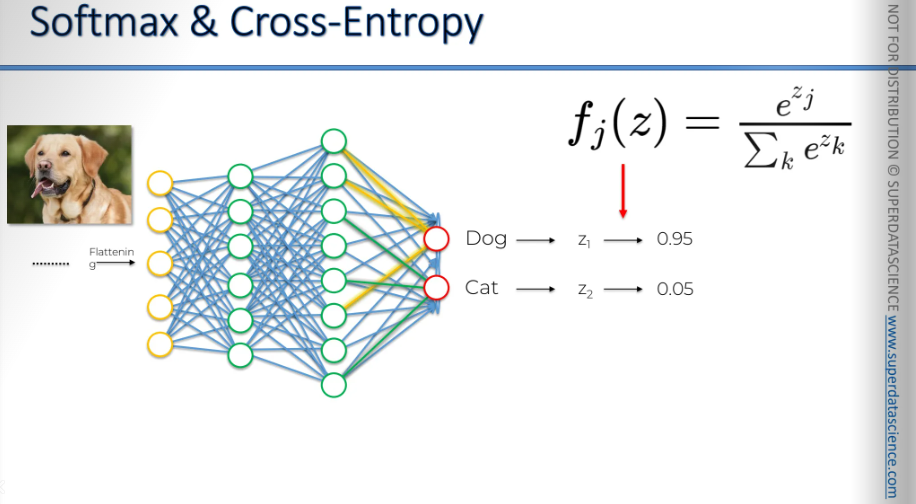
Another important point is that the softmax function works closely with something called the cross-entropy function, which is very useful for us.

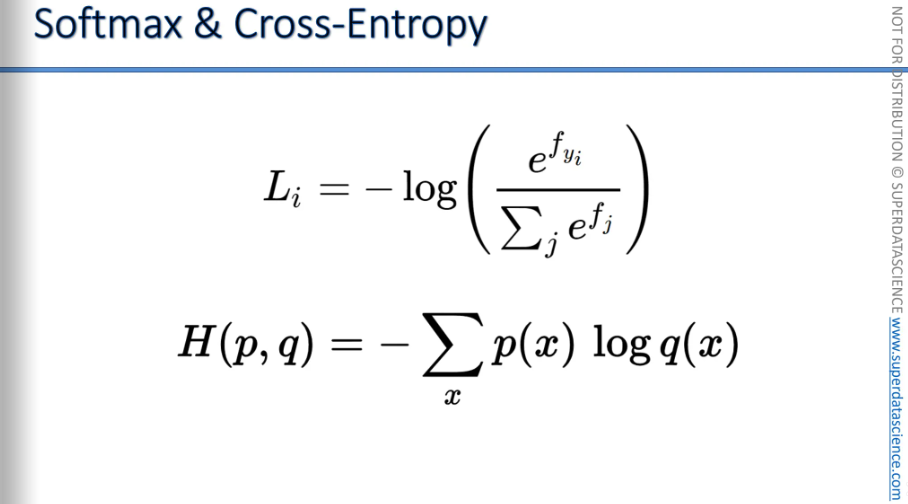
This is the formula for the cross entropy. But we will represent it with the 2nd formula (it won’t change the final result, this is just easier to calculate)

What is cross-entropy?

Cross-entropy is a function used in neural networks. Previously, in artificial neural networks, we used a function called the mean squared error (MSE) as the cost function to evaluate our network's performance. Our goal was to minimize the MSE to optimize performance.

In convolutional neural networks, we can still use MSE, but after applying the softmax function, the cross-entropy function is a better choice. In this context, it's no longer called the cost function; it's referred to as the loss function. While they are similar, there are slight differences in terminology and meaning. For our purposes, they serve the same role. The loss function is something we aim to minimize to maximize the network's performance.

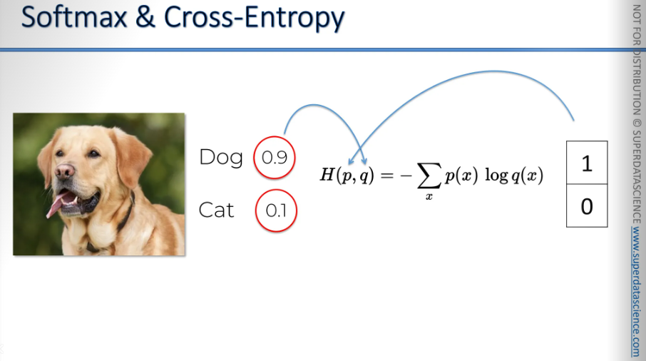
So, let's say we put an image of a dog into our network. The predicted value for the dog is 0.9. Since this is during training, we know the label is a dog. In this case, you need to plug these numbers into your formula for cross-entropy.

Here's how you would do it:

The values on the left go to the variable q, which is under the logarithm on the right side, and the values from the right go into P. It's important to remember which one goes where because if you mix them up, you don't want to take a logarithm of a 0 value or a logarithm from a 1.

Let's say we have two neural networks, and we input an image of a dog. We know this is a dog and not a cat.

Then, we have another image of a cat, indeed a cat and not a dog.

Next, we have a strange-looking animal, which is actually a dog, not a cat, if you look closely. So, we want to see what our neural networks will predict.

In the first case:

Neural Network 1 predicts: 90% dog, 10% cat. Correct.
Neural Network 2 predicts: 60% dog, 40% cat. Worse, but correct.

Second example:

Neural Network 1 predicts: 10% dog, 90% cat. Correct.
Neural Network 2 predicts: 30% dog, 70% cat. Correct, but not as good.

Finally, in image 3:

Neural Network 1 predicts: 40% dog, 60% cat. Incorrect.
Neural Network 2 predicts: 10% dog, 90% cat. Incorrect and worse.

The main point is that even though both networks were wrong in the last example, across all three images, Neural Network 1 performed better than Neural Network 2. In the last case, Neural Network 1 gave a 40% chance for a dog, while Neural Network 2 only gave a 10% chance. Therefore, Neural Network 1 is consistently outperforming Neural Network 2.

Now, let's look at the functions that can measure performance, which we've talked about before. Let's put this information into a table.

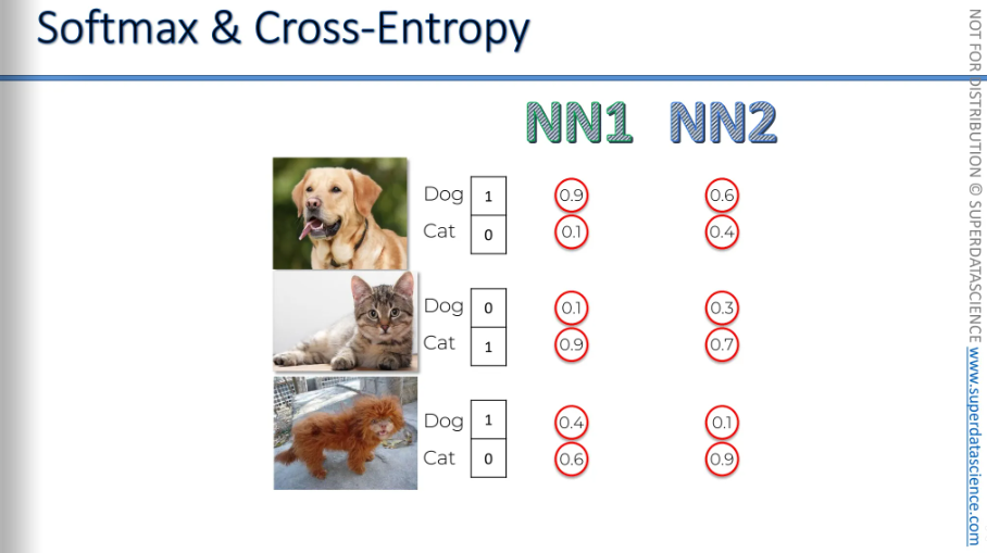
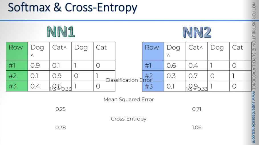
We have a table for the two neural networks. There's a column that represents the total number of tests, and in the rows, we have the probabilities they showed as well as the correct answers in binary format.

Now, what errors we can calculate from here?

The first one is the Classification Error. This simply asks, did you get it right or not? Regardless of the probabilities, it's just about whether you got it right or not. In each case, they got 1 out of 3 wrong. So, each of them has a 33% error rate. It might seem that both are performing the same, but we know NN1 is outperforming. That's why a classification error is not a good measure, especially for the back propagation.
Mean squared error: for Neural Network 1 is 25%. For Neural Network 2, it is 71%. As you can see, this is more accurate. It shows that NN1 has a lower performance error.
Cross-entropy: once again, is a formula we've discussed. You can calculate it too. It's actually easier to compute than the mean squared error. For Neural Network 1, cross-entropy is 38%, and for Neural Network 2, it is 1.06.

These calculations show that it's all possible. You can even do it on paper. These aren't very complex math problems; they're quite simple. But why choose cross-entropy over mean squared error? That's a great question. Cross-entropy has several benefits that aren't obvious. For example, at the start of backpropagation, if your output value is very tiny, much smaller than the desired value, the gradient in gradient descent will be too low. This makes it hard for the neural network to start adjusting weights and moving in the right direction. Cross-entropy, with its logarithm, helps the network recognize even small errors and take action. Here's a simple way to think about it.

If you're really interested in why we use cross-entropy instead of mean squared error, search for a video by Geoffrey Hinton called "The softmax output function." He explains it very well. As the godfather of deep learning, who can explain it better? By the way, any video by Geoffrey Hinton is excellent. He has a great talent for explaining things. So, that's softmax versus cross-entropy.

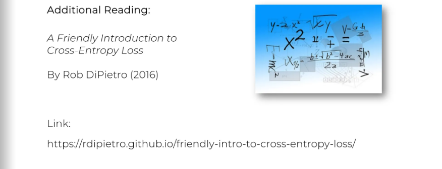
If you want a simple introduction to cross-entropy and are curious to learn more, a great article to read is A Friendly Introduction to Cross-Entropy Loss by Rob DiPietro, 2016. It's very nice, very good and easy to understand, no complicated math, good analogies and examples.

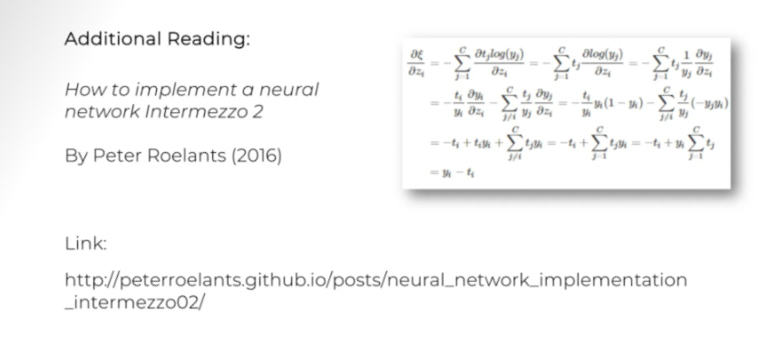
If you want to dive into the detailed math, check out an article or blog called How to Implement a Neural Network Intermezzo. The term "intermezzo" refers to an intermediate step, like a break between acts in a theater. The author, Peter Rowlands, uses it to explain steps in the process. This article is from 2016, so it's fairly recent. If you're interested in the math behind cross-entropy and SoftMax, give it a read.

CNN in python

Remember the features of the customers in the bank. Here, we're going to add a convolution layer at the beginning, which can visualize or interpret images like humans do. That's quite exciting.

I will be completing only the important here’s. other thing you will get from my GitHub repo.

We have 3 folders here.

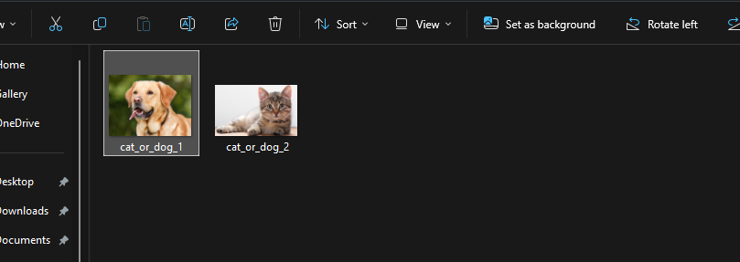
training_set consists of lots of cats and dogs image.
test_set has some cats and dogs image to check if we are right or how much right.
single_prediction has two image. 1 cat and 1 dog . It's basically production folder to detect finally if an image is cat or dog.

Data Preprocessing

we're actually going to do multiple things. First of all, we will apply transformations to all the images from the training set to avoid overfitting. Overfitting reduces accuracy drastically. But we won't apply transformations to the test set.

So, what are these transformations?

Apply some simple geometrical transformations.
Perform zooms or rotations on your images.
Apply geometrical transformations like translations to shift some of the pixels.
Rotate the images slightly.
Perform some horizontal flips.
Zoom in and zoom out on the images.

All these transformations is called Image Augmentation.

Keras API: Keras 3 API documentation [Keras is a Deep Learning library for Python, that is simple, modular, and extensible]

Check this out. It has been deprecated now!!

We will take a part from here, a code snippet you can say. Copy and paste the first portion. Then copy the 2nd portion.

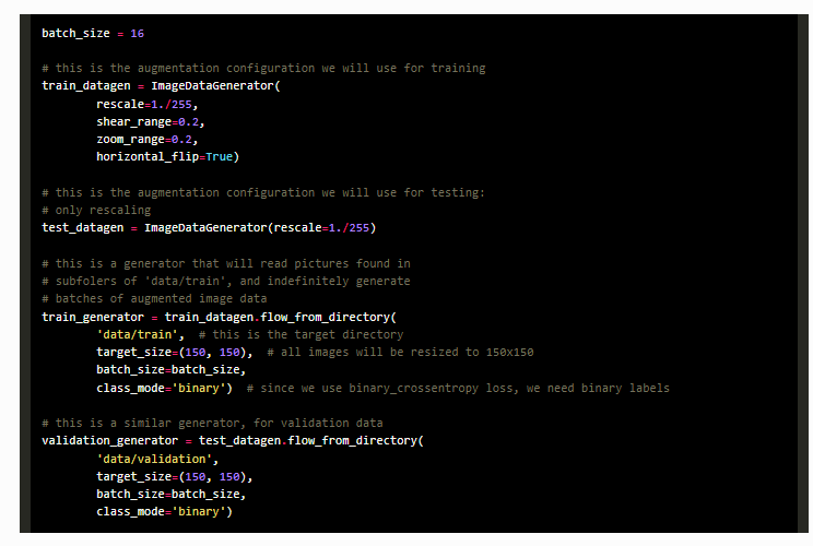
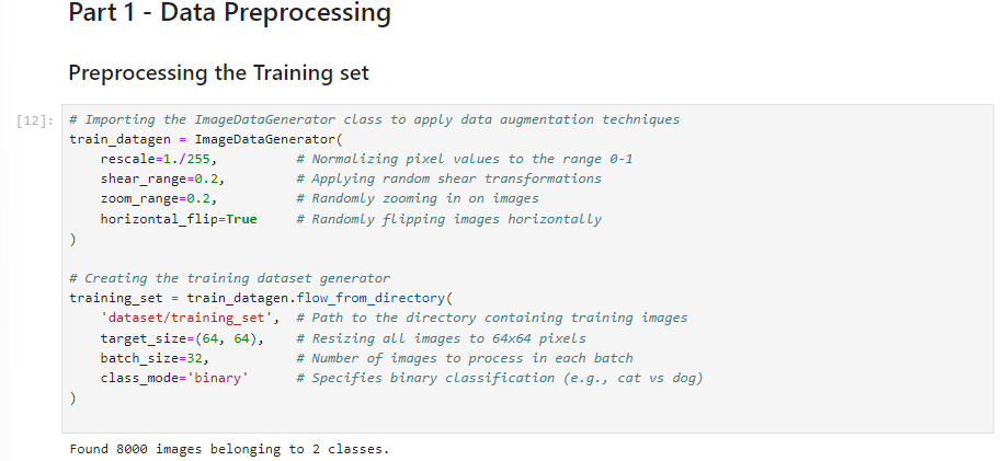
we are done with the preprocessing for training data

Now, let's do it for training data.

Note: We won't do those image augmentation for test data as our target is to check what results we get using test data. We will keep the data intact. We will just re-scale but not those data augmentation.

Now we are done with data preprocessing.

Building the CNN

Initialising the CNN:

Step 1 - Convolution:

We will add layers here

The Conv2D class, helps build a fully connected layer, is part of the same module, which is the layers module from the Keras library in TensorFlow.
On a general rule, before reaching the output layer, we want a rectifier activation function. So, for this activation, we'll choose the ReLU parameter, which corresponds to the rectifier activation function.
Since we're working with colored images, they are in three dimensions, corresponding to the RGB color code. We resized our images to 64 x 64 in part one, so the input shape of our images will be 64, 64, and 3. If we were working with black and white images, we would have one instead of three.
You can find many architectures of convolutional neural networks online. There are various types of CNN but we will use the classical one which consists of 32 layers in the 1st layers and then another 32 filters in 2nd convolutional layer. (I remind you that this is an art. Feel free to try any architecture you like; you might get better results.)
Also, we will set kernel_size as 3 which means the filter (feature detector) will be of size 3*3

Those are the essential parameters we need to enter.

Step 2 - Pooling

I recommend to work with when applying, max pooling, set the size = 2.
strides = number of frames that is shifting. In our case it’s 2×2 pixels. Again, it’s recommended. It’s the default value

Adding a second convolutional layer:

Copy and paste the step 1 and step 2. Just remove input_shape = [64,64,3] cause this is only while creating the first layer.

Step 3 - Flattening:

Step 3 does not requires any parameters.

Step 4 - Full Connection:

units = number of hidden layers.
My recommendation is to use a rectifier activation function until you reach the final output layer.

Step 5 - Output Layer:

We need to add the final output layer, which will still be fully connected to the previous hidden layer.
units = in final output it is definitely 1. We are working with binary so we only need one neuron to tell the answer
Activator function = Sigmoid is recommended.

Training the CNN

We have finished building the brain, which includes the AI's eyes (convolutional layers). Now, we are going to make that brain smart by training the CNN on all our training set images.

We're going to evaluate our model on the test set. We'll train our CNN over 25 epochs.

Compiling the CNN:

We will compile our CNN into an optimizer, loss function and some metrics.

optimizer = We're going to choose the adam optimizer again to perform stochastic gradient descent. This will update the weights to reduce the error between the predictions and the target.
loss function = We're going to use the same loss function, which is binary cross_entropy loss. We're using it again because we're doing the same task: binary classification.
metrics = And for the metrics, we're going to choose accuracy, because it's the most relevant way to measure how well a classification model performs, which is exactly the case with our CNN.

Training the CNN on the Training set and evaluating it on the Test set:

Don’t run this now. Run after making a single prediciton

x = training set to which we applied this image data generated tool,

to perform image augmentation.
validation data = the test set, that will be the value of the parameter.
epochs = inevitable argument when training a deep neural network.

I started with 10 epochs, but it wasn't enough. Then I tried 15, still not enough. Finally, 25 epochs worked perfectly. The accuracy converged on both the training and test sets. We'll use 25 epochs, but you can increase it if you have time. Running 25 epochs should take about 10 to 15 minutes.

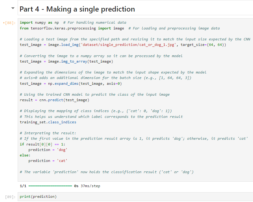
Making a single prediction

import numpy as np
from tensorflow.keras.preprocessing import image
test_image = image.load_img('dataset/single_prediction/cat_or_dog_1.jpg', target_size = (64, 64))
test_image = image.img_to_array(test_image)
test_image = np.expand_dims(test_image, axis = 0)
result = cnn.predict(test_image)
training_set.class_indices
if result[0][0] == 1:
  prediction = 'dog'
else:
  prediction = 'cat'

Final Demo

You will need to do this in Anaconda. Download Anaconda. As you have noticed, I have done the whole code in Anaconda. Even if you have done this on colab, get the code cells on notebook from colab.

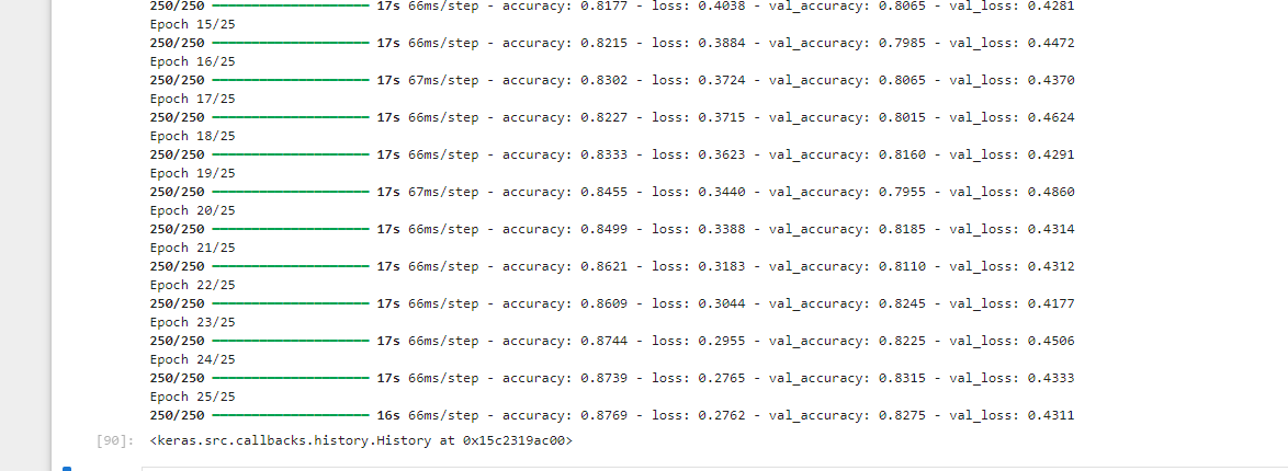
We achieved a final accuracy of 87% on the training set and 82% on the test set, which is excellent. Remember, if we hadn't done the image augmentation in part one, we could have ended up with a training set accuracy of around 98% or 99%, indicating overfitting, and a lower test set accuracy of about 70%. This is why I emphasize that image augmentation is essential.

And now, let's test our model in production by making a prediction on a single image.

Before we run this, let's make sure we know what we're predicting. Go back to your folder, navigate to the dataset, and remember, those single images are in the single prediction folder.

We'll start with the image named "cat_or_dog_1," which contains a dog. Now, we'll check if our CNN can correctly predict that there is indeed a dog in this image.

Print the single prediction cell then print(prediction); let’s really hope our model can recognize the dog as a dog …. ……and

Perfect! Our CNN successfully predicted the image.

Now for the cat:

This is the cat

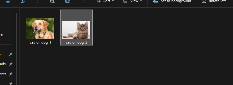
Make sure to update the file path

Run your code.

Print your prediction.

And perfect!!! CNN successfully recognized cat as a cat!

However, i took some images from the test set, rename and tried them on. And it could tell weather it’s a cat ‘ or dog.

You can try this too!

Get your code here.

ML Chapter 8.2 : Deep Learning

Table of contents