DDPM Explained for Dummies!

The following blog post is meant to be a companion post for understanding the math of the paper: Denoising Diffusion Probabilistic Models. There are a lof of other blogposts that tackle this in a more elegant and structured manner. Most of them are listed in the reference section. This post is meant to be a Hitchhiker’s Guide to the Math of DDPM Models.

What is a Diffusion Process?

Think of dropping a bottle of ink in a cup of water—first, drop by drop, then all at once. Pretty soon, the cup will be the same color as the ink. Now, think about removing each drop of ink from the cup to get the clear water back. Impossible, right?

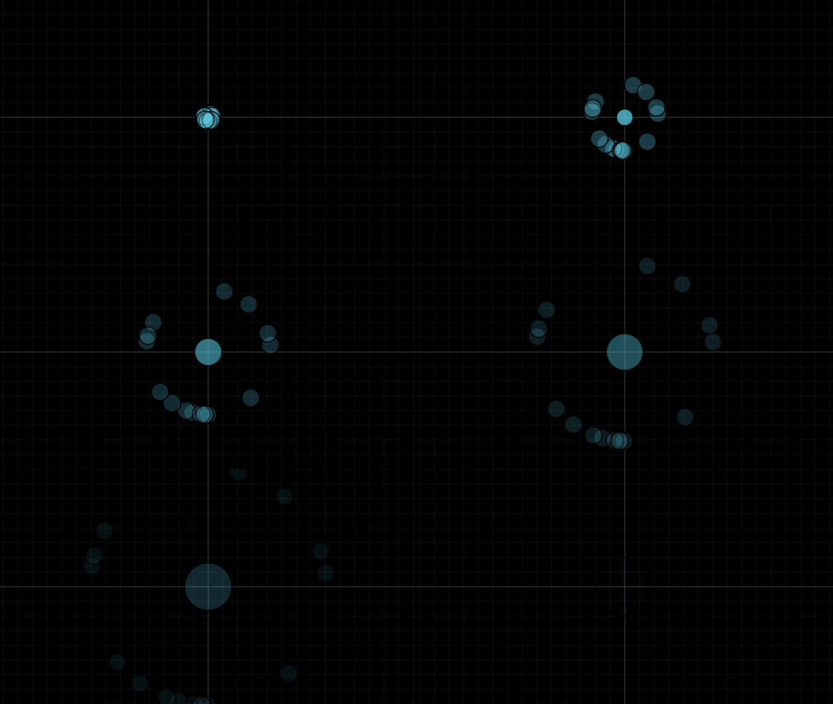
But imagine for a second you can do this. How does that help you? Well, it doesn’t until you realize that the cup of clear water you started with is not the same one you end up with. The two cups will resemble each other, but their minute properties will differ.

Diffusion Models work the same way.

1. You take an image (your clear cup of water)

2. And then add noise to it (drops of ink)

3. Till the image is just noise (fully inked cup of water)

4. Now remove the noise from the image (remove the drops of ink)

5. Till you get the same image back (original cup of clear water)

Now, if you close your eyes and think of a way to diagrammatically express this, you will most likely arrive at the following figure.

This looks an awful lot like a VAE (Variational Auto Encoder).

In a way, Diffusion models can be seen as latent variable models. Latent refers to a hidden continuous feature space.

In practice, they are formulated using a Markov chain of T steps.

Forward Diffusion Process - Noise Addition

Given a data point sampled from the real data distribution, we can define the forward diffusion process by adding noise to it.

$$q(x) = \text{Data Distribution}$$

$$x_0 = \text{Original Image}$$

$$x_T= \text{Image at time step T}$$

Here x_T is the Image at time step T(with noise added), initially, T was set to 1000.

Note: x_T will always be an image with a little bit more noise than x_(T-1)

$$q(x_t | x_{t-1}) = \text{The forward process}$$

This takes in an image and returns an image with a little bit more noise added.

Specifically, at each step of the Markov chain, we add Gaussian noise with variance t to xt-1, producing a new latent variable xt with distribution q(xt | xt-1). The diffusion process can be formulated as below:

$$q(x_t | x_{t-1}) = N(x_t, \sqrt{1 - \beta_t} x_{t-1}, \beta_t I)$$

If you are frightened by the formula, don’t worry; it is just scary-looking notations and we will learn the notations in a second.

List of Notations and their meaning

$$x_t= \text{Output}$$

Here this can mean the output or a more noisy image

$$q(x_t | x_{t-1}) = \text{The forward process}$$

This represents the probability distribution of the noisy image x_t at a specific step t

$$\beta_t = \text{Variance}$$

$$\sqrt{1 - \beta_t} =\text{Mean of Noise}$$

$$I = \text{Identity Matrix}$$

What is happening with Beta_t?

Let us try to break that down in the most simple way:

$$\sqrt{1 - \beta_t x_{t-1}}$$

This term scales the previous image x_(t-1)by a factor slightly less than 1.

This factor is:

• $$\sqrt{1 - \beta_t }$$

  The value of t is between 0 and 1 and controls the amount of noise added at each step.

• As t increases (more steps), t gets larger, so this term gets smaller, pushing the image towards zero.

The original paper (2020 -DDPM) had the following range for

beta_start = 0.0001 and beta_end = 0.02

This works to keep the variance in a lower bound. In simpler terms, this formula gradually injects noise into an image by:

• Slightly weakening the previous version of the image at each step.

• Adding random noise scaled by a factor that increases with each step.

By repeating this process for many steps (increasing t), the image becomes increasingly noisy, essentially losing its details

This gives us an idea of what to do to apply a forward step:

• Pass the image from the previous step

• Add noise of a particular mean and variance (determined by )

• Keep increasing the as per a schedule thus scaling down the image

• Obtain a progressively noisier image

So now, what do we do to apply this forward process for 1000 steps (remember T=1000

One answer is to do this for a thousand steps, which might seem tempting, but exploring math gives us a better (read easier) way to do this.

Let us revisit the equation first:

$$q(x_t | x_{t-1}) = N(x_t, \sqrt{1 - \beta_t x_{t-1}}, \beta_t I)$$

Now let's substitute the following

$$\sqrt{\beta_t} \rightarrow \alpha_t$$

Let us also define a cumulative product of all alphas

For the following:

$$t = N; \quad \alpha_N = \alpha_1. \alpha_2. \alpha_3. \alpha_4 \ldots \alpha_N$$

The mathematical way to write this is:

$$\bar{\alpha}t = \prod{N=1}^{t} \alpha_N$$

Now let us rewrite the above formula as follows using the reparameterization trick.

$$N(\mu, \sigma^2) = \mu + \sigma \cdot \varepsilon$$

Back to the formula at hand

$$q(x_t | x_{t-1}) = N(x_t, \sqrt{1 - \beta_t x_{t-1}}, \beta_t I)$$

$$= \sqrt{1 - \beta_t x_{t-1}} + \sqrt{\beta_t} \varepsilon$$

Here is sampled from a Normal distribution with Mean = 0 and Standard Deviation = 1. We can view a Normal Distribution in the diagram below.

Now, we can rewrite the above equation with

$$= \sqrt{1 - \beta_t x_{t-1}} + \sqrt{\beta_t} \varepsilon_t$$

$$= \sqrt{\alpha_t x_{t-1}} + \sqrt{1 - \alpha_t} \varepsilon_t$$

We can directly go from time step t-1 to t-2 , all the way to t=0, by chaining the alphas.

$$= \sqrt{\alpha_t \cdot \alpha_{t-1} \cdot x_{t-2}} + \sqrt{1 - \alpha_t \cdot \alpha_{t-1}} \cdot \varepsilon_{t-1}$$

$$= \sqrt{\alpha_t \cdot \alpha_{t-1} \cdot \alpha_0} \cdot x_0 + \sqrt{1 - \alpha_t \cdot \alpha_{t-1} \cdot \alpha_0} \cdot \varepsilon$$

If only we had a way to collapse the alphas into a cumulative term, but wait, we do have that:

$$= \sqrt{\bar{\alpha}_t} x_0 + \sqrt{1 - \bar{\alpha}_t} \varepsilon_t$$

Reverse Diffusion Process - Noise Removal

p(xt-1|xt) = The reverse process, where a more noisy image is passed to the function and out comes a less noisy image. In this case, the function is a model (specifically a U-Net model, but we can learn about that later)

We can express the formula in the following way:

$$p(x_{t-1}|x_t) = N(x_{t-1}; \mu_{\theta}(x_t, t), \Sigma_{\phi}(x_t, t))$$

List of Notations and their Meaning

$$x_t = \text{More Noisy Image}$$

$$x_{t-1} = \text{Less Noisy Image}$$

$$p(x_{t-1}|x_t) = \text{The Reverse Process}$$

In this case, we will have two neural networks (μ and Σ) that parameterize the normal distribution which we can sample from to get x_t-1, the more

$$\mu_\theta(x_t,t)=\text{Mean of the normal distribution, parameterized by neural network θ}$$

$$\Sigma_\phi(x_t,t)= \text{Variance of the normal distribution, parameterized by neural network} \phi$$

In practice, the variance term Σφ(x_t, t) is often set to a fixed schedule, simplifying the model.

The ultimate goal is to train a neural network to accurately predict the noise difference between two-time steps, enabling the effective denoising process.

Arriving at a Formula

Let us begin with the core structure that connects the entire process. The Loss Function of the Diffusion Model. But before we do, here is a short mathematical note that might come in handy

ELBO Formulation

The variational lower bound or Evidence Lower Bound (ELBO) can be expressed as follows:

$$\mathcal{L} = \mathbb{E}_{q(z)}[\log q(z) - \log p(z, x)]$$

Here's a breakdown of the equation:

• L: This represents the variational lower bound itself.

• Eq(z)[...]: This denotes the expectation over the variational distribution q(z). Expectation refers to the average value of a function evaluated for each possible outcome of a random variable.

• q(z): This is the variational distribution, which approximates the true intractable posterior distribution p(z|x).

• log q(z): This is the logarithm of the variational distribution.

• log p(z,x): This is the logarithm of the joint probability distribution p(z,x), where z is the latent variable and x is the data point.

Loss Function

Loss Function = negative Log Likelihood of the following term:

$$-log(p(x_0))$$

But remember this is the reverse process and we must start at x_T and move back to x_0, so the probability of x_0 will depend on all previous terms such as x_1, x_2, x_3,..., x_T-1,x_T. This makes it incredibly complex to predict the probability.

To solve this problem, we can compute the Variational Lower Bound for this objective and arrive at a more reasonable formula.

How does the reasonable formula look? Well, a little bit like this:

$$-\log(p_{\theta}(x_0)) \leq -\log(q(x_0)) + D_{KL}(q(x_{1:T}|x_0)||p_{\theta}(x_{1:T}|x_0))$$

Now if you are thinking about giving up, at this point, don’t. Because this is just scary-looking syntax and soon we will simplify it to simpler-looking syntax.

Now all this equation is saying is:

-p -p + DKL(something)

This seems reasonable, it means the negative log-likelihood of x_0 will always be less than the negative log-likelihood of x_0 added with a certain term called DKL.

So the first thing we need to learn about is DKL. It is the symbol for expressing something called KL Divergence.

Before that let us digress a bit:

• Let's say we have a function f(x) that we can’t compute.

• If we can prove that some function g(x) is always smaller than f(x)

• Then theoretically by maximizing g(x), we can be certain that f(x) also increases.

Let us look at two distributions in the following Figure.

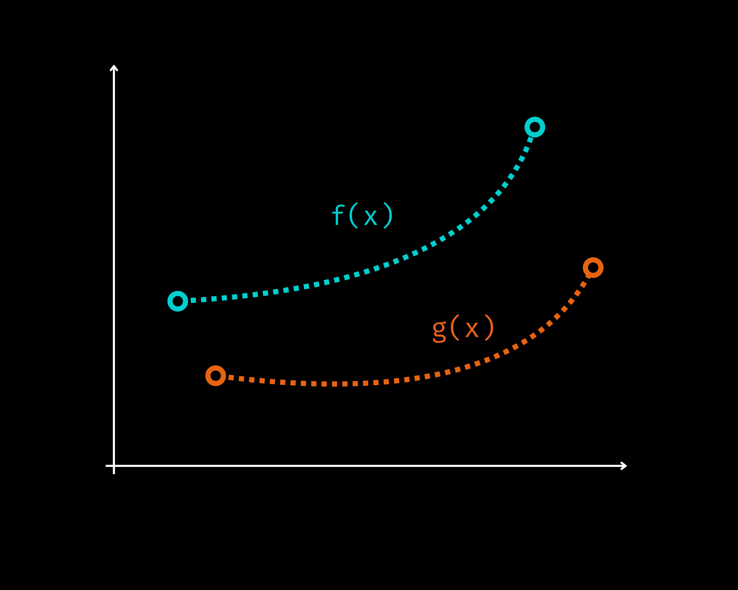
Two distributions f(x) and g(x) where g(x) < f(x) always

In this case, this is ensured by subtracting the KL divergence. So what exactly is KL Divergence?

KL Divergence Formulation

$$D_{KL}(p||q) = \int_x p(x) \log \frac{p(x)}{q(x)} dx$$

Removing uncomputable terms

But we have a problem, we have the same term that we previously mentioned is uncomputable for us

$$-\log(p_{\theta}(x_0)) \leq -\log(q(x_0)) + D_{KL}(q(x_{1:T}|x_0)||p_{\theta}(x_{1:T}|x_0))$$

So let’s start with the other term

$$-\log(p_{\theta}(x_0)) \leq -\log(q(x_0)) + D_{KL}(q(x_{1:T}|x_0)||p_{\theta}(x_{1:T}|x_0))$$

$$= \log(\frac{q(x_{1:T}|x_0)}{p_\theta(x_{1:T}|x_0)})$$

Applying the Bayesian Rule to just the denominator:

$$p_{\theta}(x_{1:T}|x_0) = \frac{p_{\theta}(x_{1:T}, x_0)}{p_{\theta}(x_0)} = \frac{p_{\theta}(x_{1:T}, x_0)}{p_{\theta}(x_0)} = \frac{p_{\theta}(x_{1:T}, x_0)}{p_{\theta}(x_0)}$$

Substituting this back into the denominator of the log term we get

$$\log(\frac{q(x_{1:T}|x_0)}{p_\theta(x_{0:T})/p_\theta(x_0)})$$

Now we can pull the bottom quantity to the top using the fraction rules and split the logarithm to get:

$$\log(\frac{q(x_{1:T}|x_0)}{p_{\theta}(x_{0:T})}) + \log(p_{\theta}(x_0))$$

Now let us remember where we started, we wanted to simplify the D_KL term, so we have:

$$D_{KL}(q(x_{1:T}|x_0)||p_{\theta}(x_{1:T}|x_0)) = \log(\frac{q(x_{1:T}|x_0)}{p_\theta(x_{0:T})}) + \log(p_{\theta}(x_0))$$

Now let us plug this back into this expression:

$$-\log(p_{\theta}(x_0)) \leq -\log(q(x_0)) + D_{KL}(q(x_{1:T}|x_0)||p_{\theta}(x_{1:T}|x_0))$$

This gives us

$$-\log(p_{\theta}(x_0)) \leq \log(\frac{q(x_{1:T}|x_0)}{p_\theta(x_{0:T})})$$

Variational Lower Bound

This is the Variational Lower Bound that we want to minimize.

Now look closely at the following expression

$$\log(\frac{q(x_{1:T}|x_0)}{p_\theta(x_{0:T})})$$

The term in the numerator is just the forward process.

The term in the denominator can be rewritten as the following:

$$p_{\theta}(x_{0:T}) = p_{\theta}(x_T) \prod_{t=1}^T p_{\theta}(x_{t-1}|x_t)$$

So let's take the current lower bound and rewrite it

$$\log(\frac{q(x_{1:T}|x_0)}{p_\theta(x_{0:T})}) = \log(\frac{\prod_{t=1}^{T}q(x_t|x_{t-1})}{p(x_T)\prod_{t=1}^{T}p_\theta(x_{t-1}|x_t)}) \\$$

$$= -\log(p(x_T)) + \log(\frac{\prod_{t=1}^{T}q(x_t|x_{t-1})}{\prod_{t=1}^{T}p_\theta(x_{t-1}|x_t)}) \\$$

$$= \log(p(x_T)) + \sum_{t=1}^{T}\log(\frac{q(x_t|x_{t-1})}{p_\theta(x_{t-1}|x_t)})$$

Next, we take out the first term or t=0

$$-\log(p(x_T)) + \sum_{t=2}^{T} \log \frac{q(x_t|x_{t-1})}{p_{\theta}(x_{t-1}|x_t)} + \log \frac{q(x_1|x_0)}{p_{\theta}(x_0|x_1)}$$

Now applying Baye’s rule to the numerator of this

$$\log \frac{q(x_t|x_{t-1})}{p_{\theta}(x_{t-1}|x_t)}$$

term we get:

$$q(x_{t-1}|x_t) = \frac{q(x_{t-1}|x_t)q(x_t)}{q(x_{t-1})}$$

Conditioning on the original Image

Now imagine looking at a noisy image, being shown a less noisy image, and being asked whether it is logically the image at the next step.

You can’t tell, right? This is because the two images you are shown have a high variance. This is true for x_t-1 and x_t

One way this can be remedied is by showing the original picture, each time you are shown the two noisy images. In math language, we say this as conditioning with the original term x_0.

$$q(x_{t-1}|x_t) = \frac{q(x_{t-1}|x_t, x_0) q(x_t|x_0)}{q(x_{t-1}|x_0)}$$

Now plugging this into the equation of the lower bound we get:

$$= -\log(p(x_T)) + \sum_{t=2}^T \log \frac{q(x_t|x_{t-1})}{p_{\theta}(x_{t-1}|x_t)} + \log \frac{q(x_1)}{p_{\theta}(x_1)}$$

$$= -\log(p(x_T)) + \sum_{t=2}^T \log \frac{q(x_t|x_{t-1}) q(x_{t-1})}{p_{\theta}(x_{t-1}|x_t) q(x_{t-1})} + \log \frac{q(x_1)}{p_{\theta}(x_1)}$$

Next, we split up the summation term into two parts because it helps us in the simplification process:

$$= -\log(p(x_T)) + \sum_{t=2}^T \log \frac{q(x_t|x_{t-1}, x_{t-2})}{p_{\theta}(x_{t-1}|x_t)} + \sum_{t=2}^T \log \frac{q(x_t|x_{t-1})}{q(x_{t-1}|x_{t-1})} + \log \frac{q(x_1|x_0)}{p_{\theta}(x_0|x_1)}$$

Let us zoom into the second summation term and set T=4

$$\sum_{t=2}^4 \log \frac{q(x_t|x_{t-1}, x_0) q(x_{t-1}|x_{t-2}, x_0) q(x_{t-2}|x_{t-3}, x_0)}{q(x_{t-1}|x_{t-2}, x_0) q(x_{t-2}|x_{t-3}, x_0) q(x_{t-3}|x_{t-4}, x_0)} = \sum_{t=2}^4 \log \frac{q(x_t|x_{t-1}, x_0)}{q(x_{t-1}|x_{t-2}, x_0)}$$

Half of these terms cancel each other out leaving the above-simplified expression, for the sake of simplification the authors wanted the second summation term to be

$$\sum_{t=2}^T \log \frac{q(x_t|x_0)}{q(x_{t-1}|x_0)} = \log \frac{q(x_T|x_0)}{q(x_1|x_0)}$$

Again plugging that into the variational lower bound formula we get:

$$E = -\log(p(x_T)) + \sum_{t=2}^T \log \frac{q(x_t|x_{t-1}, x_0)}{p_\theta(x_{t-1}|x_t)} + \log \frac{q(x_T|x_0)}{q(x_1|x_0)} + \log \frac{q(x_1|x_0)}{p_\theta(x_0|x_1)}$$

Expanding the last two log terms:

$$= -\log(p(x_T)) + \sum_{t=2}^T \log \frac{q(x_t|x_{t-1}, x_0)}{p_\theta(x_{t-1}|x_t)} + \log q(x_T|x_0) - \log q(x_1|x_0) + \log q(x_1|x_0) - \log p_\theta(x_0|x_1)$$

$$= -\log(p(x_T)) + \sum_{t=2}^T \log \frac{q(x_t|x_{t-1}, x_0)}{p_\theta(x_{t-1}|x_t)} + \log q(x_T|x_0) - \log p_\theta(x_0|x_1)$$

$$= \frac{\log q(x_T|x_0)}{\log p(x_T)} + \sum_{t=2}^T \log \frac{q(x_t|x_{t-1}, x_0)}{p_\theta(x_{t-1}|x_t)} - \log p_\theta(x_0|x_1)$$

Rewriting this as a KL Divergence we get:

$$= D_{KL}(q(x_T|x_0)||p(x_T)) + \sum_{t=2}^T D_{KL}(q(x_t|x_{t-1}, x_0)||p_{\theta}(x_{t-1}|x_t)) - \log(p_{\theta}(x_0|x_1))$$

Arriving at the Objective Function

And that is our objective that we want to minimize, yes this feels like a step backward in terms of simplification, but let us zoom in and see which terms we can minimize or ignore for the sake of simplicity.

For example, the first term

$$D_{KL}(q(x_T|x_0)||p(x_T))$$

will always be low and can be ignored as far as finding the objective function for the loss is concerned because:

• q(x_T|x_0) is just the forward process with no learnable parameters and will eventually converge to random noise

• p(x_T) is random noise sampled from a Gaussian distribution

Thus reformulating we have the following:

$$= \sum_{t=2}^T D_{KL}(q(x_t|x_{t-1}, x_0)||p_{\theta}(x_{t-1}|x_t)) - \log(p_{\theta}(x_0|x_1))$$

Substituting the Mean in the KL Divergence

At this stage, it is good to recalibrate how this expression connects to the individual expressions of the forward and reverse processes, shown in the following figure.

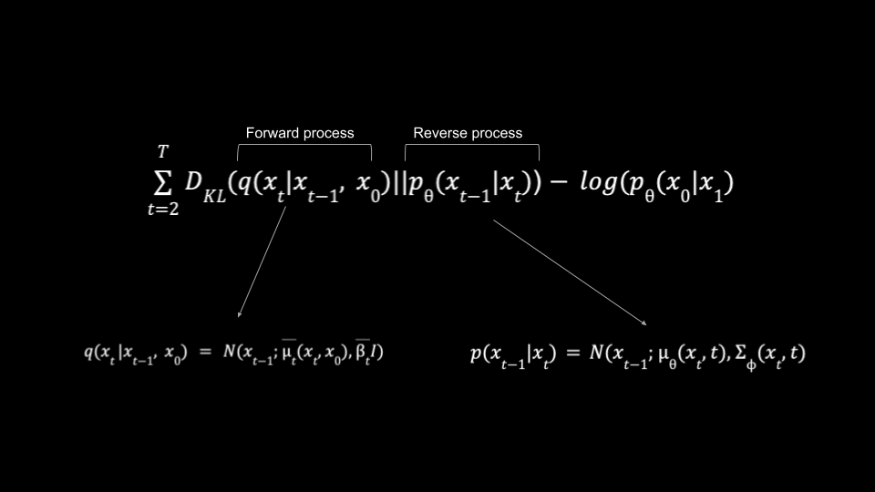
Analytically arriving at the Mean of the Reverse Process

Now let's look at the reverse process at p(x_t-1|x_t), We already know that

$$p(x_{t-1}|x_t) = N(x_{t-1}; \mu_{\theta}(x_t), \Sigma_{\phi}(x_t))$$

We can ignore the variance term since it has a fixed schedule, so we can rewrite this as:

$$p(x_{t-1}|x_t) = N(x_{t-1}; \mu_{\theta}(x_t), \beta I)$$

So this means we need a neural network to predict the mean of the noise. Now let us express the forward process in a similar style.

Analytically arriving at the Mean of the Forward Process

We also know that the forward process q(x_t|x_t-1, x_0) has an expression like the following:

$$q(x_t|x_{t-1}) = N(x_t, \sqrt{1-\beta_t}x_{t-1}, \beta_t I)$$

For the sake of making this similar, let us rewrite the above expression while conditioning on x_0 and using a function like µ_t

$$q(x_t|x_{t-1}, x_0) = N(x_t; \overline{\mu}_{\phi}(x_t, x_0), \overline{\beta}_t I)$$

Deriving the terms µ_t, and β_t will make this unnecessarily stretched out, so let us leave them as they are:

$$\overline{\mu}t(x_t, x_0) = \frac{\sqrt{\alpha_t(1-\overline{\alpha}{t-1})}}{1-\overline{\alpha}t}x_t + \frac{\sqrt{\overline{\alpha}{t-1}\beta_t}}{1-\overline{\alpha}_t}x_0$$

$$\overline{\beta}t = \frac{1-\overline{\alpha}{t-1}}{1-\overline{\alpha}_t}\beta_t$$

We can safely ignore the β_t term since it is fixed, let us instead focus on µ_t(X_t,X_0)

We know that

$$\log(\frac{q(x_{1:T}|x_0)}{p_\theta(x_{1:T}|x_0)})$$

So,

$$x_0 = \frac{1}{\sqrt{\alpha_t}}(x_t - \sqrt{1-\overline{\alpha_t}}\epsilon)$$

Plugging this into µ_t we have:

$$\overline{\mu}_t(x_t, x_0) = \frac{1}{\sqrt{\alpha_t}}(x_t - \frac{\beta_t}{\sqrt{1-\alpha_t}}\epsilon)(\frac{1}{\sqrt{\alpha_t}}(x_t - \sqrt{1-\overline{\alpha}_t}\epsilon))$$

$$\overline{\mu}t(x_t, x_0) = \frac{\sqrt{\alpha_t(1-\overline{\alpha}{t-1})}}{1-\overline{\alpha}t}x_t + \frac{\sqrt{\overline{\alpha}{t-1}\beta_t}}{1-\overline{\alpha}_t}(x_t - \sqrt{1-\overline{\alpha}_t}\epsilon)$$

$$\overline{\mu}_t(x_t, x_0) = \frac{1}{\sqrt{\alpha_t}}(x_t - \frac{\beta_t}{\sqrt{1-\alpha_t}}\epsilon)$$

Essentially this means we are just subtracting random scaled noise from x_t

Expressing the Mean of the Reverse Process as a similar expression

Now let us again go back to how the forward and reverse diffusion process connects to the variational lower bound expression. But this time let us also look at the Figure and try to figure out what is in the respective equations.

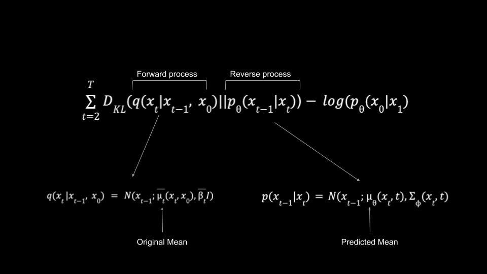
Now something funny happens here, in the reverse process:

$$p(x_{t-1}|x_t) = N(x_{t-1}; \mu_{\theta}(x_t, t), \beta I)$$

We realize that must predict the noise at time step t, given the x_t as an input to the model

Now do we have a formula where we can plug in the time step t and x_t as an input to the model. Yes, we do!

Remember for the forward process we have derived:

$$\overline{\mu}_t(x_t, x_0) = \frac{1}{\sqrt{\alpha_t}}(x_t - \frac{\beta_t}{\sqrt{1-\overline{\alpha}_t}}\epsilon)$$

So we can write as:

$$\mu_{\theta}(x_t, t) = \frac{1}{\sqrt{\alpha_t}}(x_t - \frac{\beta_t}{\sqrt{1-\overline{\alpha}t}}\epsilon{\theta}(x_t, t))$$

Here we just need a parameterized neural network ε_(x_t,t) that takes in the noisy image and the time step t and gives us the noise.

Deriving x_t-1

Now from our previous formula for the reverse process, we have:

$$p(x_{t-1}|x_t) = N(x_{t-1}; \mu_{\theta}(x_t, t), \beta I)$$

Since we already have the formula for substituting we get:

$$= N(x_{t-1}; \frac{1}{\sqrt{\alpha_t}}(x_t - \frac{\beta_t}{\sqrt{1-\overline{\alpha}t}}\epsilon{\theta}(x_t, t)), \beta I)$$

Now we can apply the reparametrization trick again and get the following value for:

$$x_{t-1} = \frac{1}{\sqrt{\alpha_t}}(x_t - \frac{\beta_t}{\sqrt{1-\overline{\alpha}t}}\epsilon{\theta}(x_t, t)) + \sqrt{\beta_t}\epsilon$$

Further Simplifying the Objective Function

Now focusing back on our objective function:

$$\sum_{t=2}^T D_{KL}(q(x_t|x_{t-1}, x_0)||p_{\theta}(x_{t-1}|x_t)) - \log(p_{\theta}(x_0|x_1))$$

Let us single out the KL Divergence part, the authors resolved to simplify this into a simple mean squared error as shown in the following Figure.

So we can write KL Divergence term as:

$$\frac{1}{2\sigma_t^2}\lVert \overline{\mu}t(x_t, x_0) - \mu{\theta}(x_t, x_0) \rVert^2$$

This simplifies matters a lot, again we can plug the values here to get:

$$\frac{1}{2\sigma_t^2}\lVert \frac{1}{\sqrt{\alpha_t}}(x_t - \frac{\beta_t}{\sqrt{1-\overline{\alpha}_t}}\epsilon) - \frac{1}{\sqrt{\alpha_t}}(x_t - \frac{\beta_t}{\sqrt{1-\overline{\alpha}t}}\epsilon{\theta}(x_t, t)) \rVert^2$$

Which can be simplified further into:

$$\frac{\beta_t^2}{2\sigma_t^2 \alpha_t(1-\overline{\alpha}t)}\lVert \epsilon - \epsilon{\theta}(x_t, t) \rVert^2$$

So the final expression becomes:

$$\frac{\beta_t^2}{2\sigma_t^2 \alpha_t(1-\overline{\alpha}t)}\lVert \epsilon - \epsilon{\theta}(x_t, t) \rVert^2 - \log(p_{\theta}(x_0|x_1))$$

The authors also considered the -log(p(x_0|x_1) to be a component of the prediction from the model rather than deriving its expression.

So the final objective function is:

$$\frac{\beta_t^2}{2\sigma_t^2 \alpha_t(1-\overline{\alpha}t)}\lVert \epsilon - \epsilon{\theta}(x_t, t) \rVert^2$$

Formally in the paper, this is expressed as:

$$L_{obj} = E_{t, x, \epsilon} [\frac{\beta_t^2}{2\sigma_t^2\alpha_t(1-\overline{\alpha}t)}\lVert \epsilon - \epsilon{\theta}(\sqrt{\alpha_t}x_t + \sqrt{1-\overline{\alpha}_t}\epsilon, t) \rVert^2]$$

Now you already know that the scary-looking E is simply the expectation of the random variable. That is just a fancy way of saying what the expected value of the objective function or loss would be at each time step, given the initial image and the noise.

Oh and also if you are afraid of the scary-looking alphas, remember earlier where we got:

$$x_t = \sqrt{\overline{\alpha}_t}x_0 + \sqrt{1-\overline{\alpha}_t}\epsilon$$

Summing Up (Literally)

At this juncture, it is probably best to revisit our original goal:

At the end of this entire math circus what we have with us are two very important formulas:

$$L_{obj} = E_{t, x, \epsilon} [\frac{\beta_t^2}{2\sigma_t^2\alpha_t(1-\overline{\alpha}t)}\lVert \epsilon - \epsilon{\theta}(\sqrt{\alpha_t}x_t + \sqrt{1-\overline{\alpha}_t}\epsilon, t) \rVert^2]$$

The objective function allows the use of a neural network to predict the noise at each time step.

$$x_{t-1} = \frac{1}{\sqrt{\alpha_t}}(x_t - \frac{\beta_t}{\sqrt{1-\overline{\alpha}t}}\epsilon{\theta}(x_t, t)) + \sqrt{\beta_t}\epsilon$$

Another formula that allows us to create the image for the subsequent time steps from the current time steps.

Congratulations! 🎉

References:

• Aritra Roy Gosthipaty ‘s work on Explaining DDPM Models

• PyImageSearch Course on Build an AI Image Generator

• https://www.youtube.com/watch?v=HoKDTa5jHvg

• https://www.youtube.com/watch?v=a4Yfz2FxXiY&t=1195s

• https://www.youtube.com/watch?v=HxQ94L8n0vU&t=290s

• https://theaisummer.com/diffusion-models/#approximating-the-reverse-process-with-a-neural-network

• https://magic-with-latents.github.io/latent/posts/ddpms/part3/

• https://mr-easy.github.io/2020-04-16-kl-divergence-between-2-gaussian-distributions/