Learning Parametric Partial Differential Equations using Fourier Neural Operator
 Pietro Zanotta
A variety of problems in applied science revolve about solving systems of parametrized partial differential equations. Such systems often exhibit complex and non-linear behaviour and mesh-based methods might therefore require an incredibly fine discretization to precisely capture the model. However, traditional numerical solvers come with a trade-off since coarse grids are fast but less accurate, while fine grids are accurate but slow, which means that such problems might pose a non-trivial issue to traditional solvers.
For this reason, researchers developed a whole new family of methods which can directly learn the trajectory of the family of equations from the data, resulting in faster approximation of the solution of such PDEs.
This post discusses a specific data-driven approach to approximate parametric PDEs using a specific neural architecture called Fourier Neural Operator (FNO) and concludes presenting a quantum-enhanced version of the FNO.
Learning Neural Operators
To properly understand Fourier Neural Operator, a brief introduction to neural operators is necessary. The idea underlying neural operators is to learn mesh-free, infinite dimensional operators with neural networks which is able to transfer solution between different meshes, doesn’t need to be trained for each parameter and doesn’t require any aprioristic knowledge of the PDE.
Let \(D\) be a bounded domain in \(R^d\) and let \(U(D, R^{d_u})\) and \(\Lambda(D, R^{d_\lambda})\) be two separable Banach spaces of function where \(R^{d_u}\) and \(R^{d_\lambda}\) are the codomains.
Assume the PDE one wish to solve is:
$$\mathcal L(u, x, \lambda) = 0$$
where:
\(\mathcal L\) is the differential operator
\(u \in U\) is the solution function
\(x\) is is the spatial-temporal variable
\(\lambda \in \Lambda\) is the function parametrizing the PDE
Moreover let \(G^\dagger: \Lambda \rightarrow U\) be a map which arise as the solution operators of parametric PDEs. Also let \(\{\lambda_j, u_j\}^n_{j=1}\) be observations (potentially noisy) s.t.
$$G^\dagger(\lambda_j) = u_j$$
The goal of the neural operator is to approximate \(G^\dagger\) with
$$G_\theta: \Lambda \times \Theta \rightarrow U$$
where \(\Theta\) is a finite-dimensional space.
Similarly to a finite-dimensional setting, one can now define a cost function
$$C : U \times U\rightarrow R$$
and seek a minimizer of the problem s.a.:
$$\text{min}{\theta \in \Theta}E\lambda\left( C\left(G_\theta\left(\lambda\right), G^\dagger\left(\lambda\right)\right)\right)$$
Of course, learning a neural operators is therefore much different than learning the solution to a PDE with a fixed parameter \(\lambda\). The large majority of methods to approximate PDEs (including traditional methods and machine learning approaches) would therefore reveal impractical if the solution of the PDE is required for different instances of the parameter \(\lambda\), that’s where neural operator’s approach offers a computational advantage.
Moreover, to work numerically with the data \(\{\lambda_j, u_j\}^n_{j=1}\), since both \(\lambda_j\) and \(u_j\) are in general functions, we assume to have access to point-wise evaluations of the two functions. Therefore, let \(D_j = \{x_1, \dots, x_n\}\) be a n-point discretization of the domain \(D\) and assume one have access to point-wise evaluations of the functions \(\lambda_j\) and \(u_j\) over \(D_j\).
Defining the Neural Operator
As proposed in [Li], the neural operator is an iterative architecture which updates the function \(v_j: D \rightarrow R^{d_v}\). The idea is to:
- represent the input \(\lambda \in \Lambda\) in a higher dimensional representation with the local transformation \(P\):
$$v_0(x) = P(\lambda(x))$$
- then the function \(v_j\) is updated as follows:
$$v_{t+1}(x):=\sigma\left(W v_t(x)+\left(\mathcal{K}(\lambda , \theta) v_t\right)(x)\right), \quad \forall x \in D$$
where:
\(\sigma\) is a non-linear activation function
\(W: R^{d_v} \rightarrow R^{d_v}\) is the bias term applied on the spatial domain
\(K: \Lambda \times \Theta_k \rightarrow \mathcal L\left(U\left(D, R^{d_v} \right), U\left(D, R^{d_v} \right)\right)\) is the kernel integral transformation and is parametrized by \(\theta \in \Theta_k\)
The kernel integral transformation moreover is the following:
$$\left(\mathcal{K}(\lambda , \theta) v_t\right)(x):=\int_D \kappa(x, y, \lambda(x), \lambda(y) , \theta) v_t(y) \mathrm{d} y, \quad \forall x \in D$$
where \(k\) is a neural network parametrized by \(\theta \in \Theta_k\) and represent the kernel function. It’s worth noticing that while the kernel function is linear the operator can learn non-linear operators thanks to the non-linear activation functions, analogously to standard neural networks.
Defining the Fourier Neural Operator
Let \(\mathcal F\) be the Fourier transform of a function \(f: D \rightarrow R^{d_v}\) and let \(\mathcal F^{-1}\) be the inverse of the Fourier transform. By imposing (i.e. making \(k\) a convolutional operator):
$$k(x,y,\lambda(x), \lambda(y), \theta) = k(x-y, \theta)$$
the kernel integral transformation becomes:
$$\left(\mathcal{K}(\lambda, \theta) v_t\right)(x)=\mathcal{F}^{-1}\left(\mathcal{F}\left(\kappa_\theta\right) \cdot \mathcal{F}\left(v_t\right)\right)(x), \quad \forall x \in D$$
and if the parametrization \(k_\theta\) happens directly in Fourier space:
$$\left(\mathcal{K}(\lambda, \theta) v_t\right)(x)=\mathcal{F}^{-1}\left(R_\theta \cdot \mathcal{F}\left(v_t\right)\right)(x), \quad \forall x \in D$$
as shown in the following picture (taken from [3]):
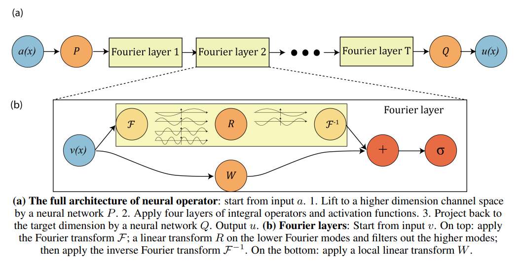
If we enforce that \(k_\theta\) is periodic, it admits a Fourier series expansion, which can be truncated at a maximum number of modes \(m_{\text{max}}\) and therefore \(R_\theta\) can be parametrized with a (\((m_{\text{max}} \times d_v \times d_v)\)-tensor.
Furthermore, once \(D \) is discretized in \(n\) points, \(v_t \in R^{n\times d_v}\). Moreover, since \(v_t\) convolves with a function with only \(m_{\text{max}}\) modes, we can truncate the the highest modes in order to have \(F(v_t) \in C^{m_{\text max} \times d_v}\).
Therefore, the multiplication for the weight tensor \(R_\theta \in C^{m_{\text{max}} \times d_v \times d_v}\) is:
$$R\cdot(\mathcal F v_t)_{m, l} = \sum_{j=1}^{d_v}R_{m, l, j}(Fv_t)_{m, j} \quad m=1,\dots, m_\text{max}, \quad j = 1, \dots, d_v$$
Invariance to discretization
It’s worth noticing that the Fourier layers are discretization-invariants since they learn from and evaluate functions which are discretized in an arbitrary way, which allows zero-shot super-resolution.
Accelerating the Fourier Neural Operator: Quantum Fourier Operator
Since the weight tensor contains \(m_{\text{max}}< n\) modes and since the complexity of inner product is \(O(m_\text{max})\), the most relevant source of computations comes from the Fourier transform and its inverse. Fourier transform complexity is in fact \(O(n^2)\) in general, but since the model deals with truncated series, the complexity is actually \(O(nm_{\text{max}})\). Therefore, substituting the Fourier transform with the fast Fourier transform (FFT), assuming a uniform discretization, can provide a speedup, being the complexity of FFT \(O(n \log n)\).
Another direction is exploit a quantum-enhanced method based on Quantum Fourier Transform to have more efficient Fourier layers.
Data encoding in the unary basis
The idea underlying Quantum Fourier Operator (QFO) is to substitute the Fourier layers defined above with a new layer exploiting quantum algorithms. Of course to make this possible the matrix \(P(\lambda(x))\) (which I’ll refer to s \(A\) from now on) has to be encoded in a quantum state to serve as the input of the new Fourier layer. The idea is to encode the data according to amplitude-encoded states, choosing as basis \(\ket {e_i}\) the quantum states with a Hamming state of 1:
$$\ket {e_i} = \ket {0\dots010\dots0}$$
Therefore given a generic \(R^{n\times m} \) matrix \(M\), it’s quantum encoding is:
$$\ket{M}=\frac 1{|M|}\sum_{i=1}^n \sum_{j=1}^m a_{i,j} \ket{e_i}\ket{e_j }$$
the circuit to load such state was developed in [7] and assuming an ideal connectivity, the circuit has depth \(O(\log(m) + 2m \log(n))\).
Unary QFT
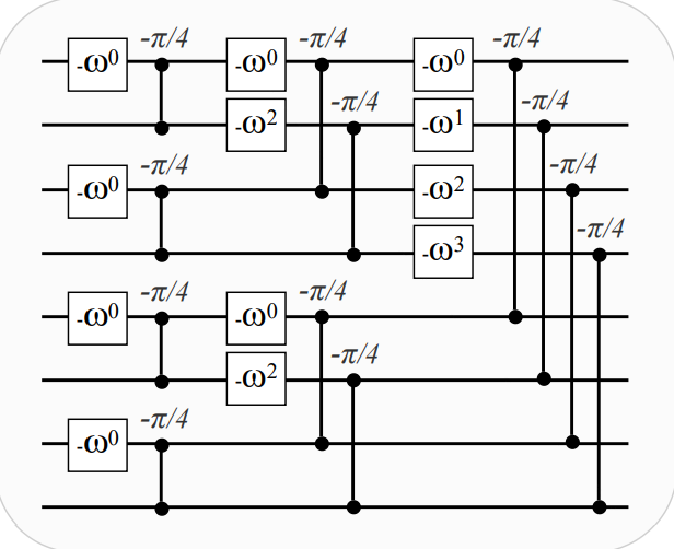
Inspired by the butterfly-shaped diagram of the FFT, one can define a unitary matrix which performs the quantum analogue of the FFT on the unitary basis whose matrix is:
$$F_n=\frac 1 {\sqrt n}\left(\begin{array}{ccccc}1 & 1 & 1 & \cdots & 1 \\ 1 & \omega & \omega^2 & \cdots & \omega^{(n-1)} \\ 1 & \omega^2 & \omega^4 & \cdots & \omega^{2(n-1)} \\ \vdots & \vdots & \vdots & \ddots & \vdots \\ 1 & \omega^{n-1} & \omega^{2 n-2} & \cdots & \omega^{(n-1)^2}\end{array}\right)$$
where \(\omega^k = e^{i\frac{2\pi k}{n}}\).
Such transformation can be implemented using phase gates and RBS gates as shown in the following picture (picture from [1]) and the depth of the resulting circuit is \(O(\log n)\):
Trainable linear transform with Quantum Orthogonal Layers
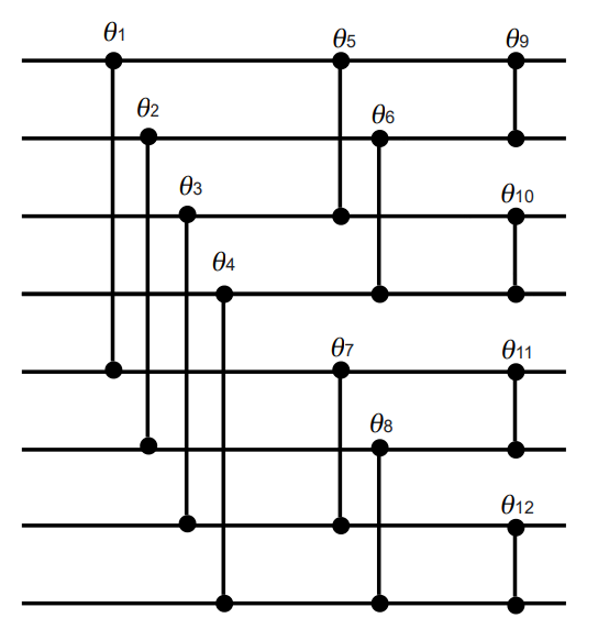
It’s now necessary to define the quantum analogue of the learnable part of the classical Fourier layer and to perform some matrix multiplication. Quantum Orthogonal Layers (from [8]) are therefore a natural choice, being parametrized and hamming-weight preserving transformations (which is a characteristics necessary to preserve since the Inverse Unitary Fourier Transform only works on the unitary basis). Several circuits in this setting exists, the butterfly circuit (which has the same layout as the one used for the Unary-QFT and that is represented in the following picture) is chosen, having \(O(n\log n) \) parametrized gates, where \(n \) is the dimension of the input vector.
Quantum Fourier Layer
Based on the above building blocks, one can define 3 quantum circuits to substitute the classical Fourier layer:
the sequential circuit
the parallel circuit
the composite circuit
The goal of all those circuit is to reproduce the result of the classical Fourier layer, which in quantum formalism is (assuming the input matrix \(A\) was normalized):
$$\ket y = \sum_i \ket{y_i}\ket{e_i} = \sum_i \sum_j y_{i j}\ket{e_i}\ket{e_j}$$
where:
$$y_{i,j} = IFT\left(\left[ w_{il}m_{il}, m_{ik}\right]\right)_j$$
with:
\(w\) being an element of \(W\)
\(m\) being an element of \(A\)
The sequential Quantum Fourier Layer
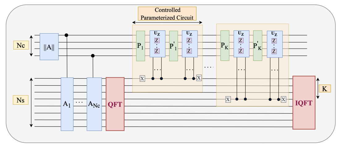
The sequential circuit starts by encoding the input matrix \(A\), resulting in:
$$\ket{\psi_0}= \sum_i \sum_j a_{ij}\ket{e_i}\ket{e_j }$$
Then to \(\ket{\psi_0}\) the Unary-QFT is applied on the second register:
$$\ket{\psi_1}= \sum_i \ket{e_i}\text{QFT}(\sum_j a_{ij}\ket{e_j }) =\sum_i \ket{e_i}(\sum_j \hat a_{ij}\ket{e_j })$$
where \(\hat a_{ij}\) is the row-wise Fourier transfor of \(A\).
After that, the trainable linear transform with quantum orthogonal layers made by \(K\) matrix multiplications has to be defined. Using the circuit depicted above (the butterfly circuit), in this sequential approach, the \(K\) parametrized quantum circuit \(P_1, \dots, P_k\) are applied sequentially on the first register.
After this the I-QFT is applied, resulting in the desired state.
The parallel Quantum Fourier Layer
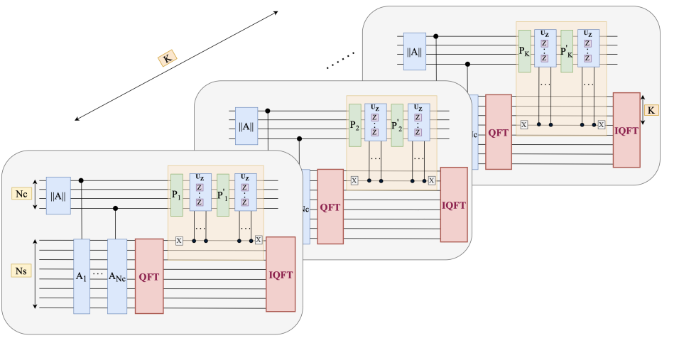
For the sequential QFL, the depth complexity of the learnable part is linear in the number of modes, which might eventually hinder learning, because of the multiplicative noise model for NISQ machines. To reduce the depth complexity and to make the algorithm more noise-resistant, an interesting modification requires to parallelise the butterfly circuits.
The composite Quantum Fourier Layer
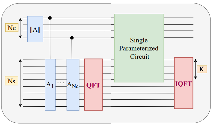
However the parallelized quantum circuit discussed in the above section requires \(K\times (d_v + n)\) independent qubits where \(K \) is the number of modes, which might end up being more than the available qubit resources.
However, one can replace the \(K\) parametrized circuits with a single parametrized circuit \(B\), as long as this new subcircuit is hamming-weight preserving and is built as:
$$B = \bigotimes_i B_i$$
where \(B_i\) correspond to the block diagonal unitary for subspace with hamming weigh \(i\).
And that's it for this article. Thanks for reading.
For any question or suggestion related to what I covered in this article, please add it as a comment. For special needs, you can contact me here.
Sources:
Subscribe to my newsletter
Read articles from Pietro Zanotta directly inside your inbox. Subscribe to the newsletter, and don't miss out.
Written by
