1. Introduction

The ability to predict loan repayment can be a game-changer for lenders and investors, providing valuable insights into risk management. In this blog, we will explore how machine learning models like Decision Trees and Random Forests can be used to predict whether a loan will be fully repaid. We’ll work with a real-world dataset from Lending Club, a platform connecting borrowers and investors.

The dataset, covering loans issued between 2007 and 2010, includes borrower details, credit scores, loan purposes, and repayment statuses. Our goal is to develop models that predict the target variable, not_fully_paid, which indicates whether a loan was not repaid in full. By the end of this blog, you’ll understand how to preprocess data, train these models, and evaluate their performance, providing actionable insights for decision-making in lending scenarios.

2. Understanding the Dataset

The dataset we’re using was sourced from Lending Club, a peer-to-peer lending platform. It represents loans issued between 2007 and 2010 and contains the following key features:

FICO: A credit score used to evaluate a borrower’s creditworthiness.
Loan Purpose: The stated reason for borrowing, such as debt consolidation, home improvement, or education.
Credit Policy: A binary feature indicating whether the borrower meets Lending Club’s underwriting criteria (1 for yes, 0 for no).
Installment: The monthly repayment amount required for the loan.
Interest Rate: The annual interest rate associated with the loan.
Not Fully Paid: The target variable we aim to predict, where 1 means the loan was not fully repaid and 0 means it was.

This cleaned dataset has already had missing values removed, making it ready for exploratory data analysis (EDA) and model training. Each row corresponds to a specific loan, providing insights into the borrower’s financial behavior and repayment history. Understanding these features is crucial as they directly influence our model’s ability to predict repayment outcomes effectively.

3. Exploratory Data Analysis (EDA)

Before training our machine learning models, we need to explore and understand the dataset’s structure and key patterns. Through visualizations and summary statistics, we aim to uncover trends and relationships that could influence loan repayment predictions.

Data Overview

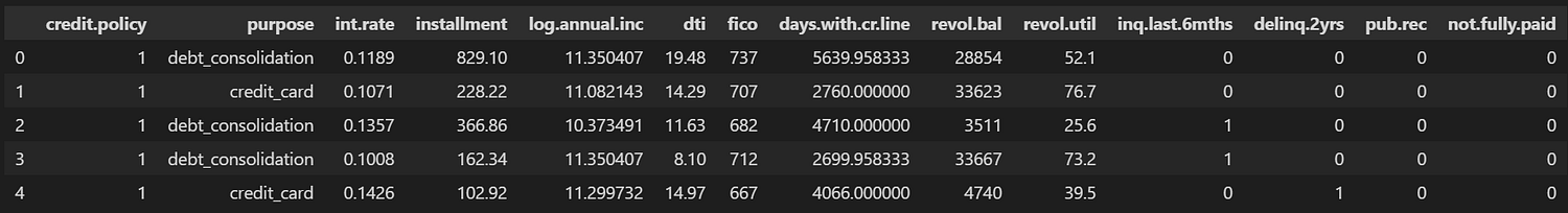
We begin by loading the dataset and inspecting its structure:

import pandas as pd

# Load the dataset
loans = pd.read_csv("loan_data.csv")
loans.head()

# Basic information 
loans.info()

<class 'pandas.core.frame.DataFrame'>
RangeIndex: 9578 entries, 0 to 9577
Data columns (total 14 columns):
credit.policy        9578 non-null int64
purpose              9578 non-null object
int.rate             9578 non-null float64
installment          9578 non-null float64
log.annual.inc       9578 non-null float64
dti                  9578 non-null float64
fico                 9578 non-null int64
days.with.cr.line    9578 non-null float64
revol.bal            9578 non-null int64
revol.util           9578 non-null float64
inq.last.6mths       9578 non-null int64
delinq.2yrs          9578 non-null int64
pub.rec              9578 non-null int64
not.fully.paid       9578 non-null int64
dtypes: float64(6), int64(7), object(1)
memory usage: 1.0+ MB

The dataset contains 9,578 rows and 14 columns, all of which have non-null values, indicating no missing data. The data types include:

6 columns with float64 type (e.g., int.rate, log.annual.inc).
7 columns with int64 type (e.g., fico, credit.policy).
1 column with object type (purpose), which is categorical.

The dataset is clean and ready for further analysis without requiring the handling of missing values. Its memory usage is approximately 1 MB.

# Basic statistics
loans.describe()

Here is a concise interpretation of the summary statistics:

credit.policy: Most borrowers meet Lending Club's underwriting criteria (mean ≈ 0.8, where 1 indicates compliance).
int.rate: The average interest rate is approximately 12.3%, ranging from 6% to 21.6%.
installment: Monthly installment payments vary widely, with a mean of 319 and a maximum of 940.
log.annual.inc: Borrowers have an average logarithmic annual income of ~10.93, which corresponds to ~$55,700 in real terms.
fico: The average FICO score is 710, ranging from 612 to 827, indicating a mix of moderate to high creditworthiness.
days.with.cr.line: Borrowers' credit lines have been open for an average of ~4,560 days (~12.5 years), with some as long as ~48 years.
dti: The average debt-to-income ratio is 12.6, with some borrowers having ratios up to 29.96.
not.fully.paid (target variable): Around 16% of loans are not fully repaid (mean ≈ 0.16), indicating the proportion of risky loans.

This dataset shows diverse borrower profiles, enabling the analysis of repayment risk based on financial behaviors and credit worthiness.

# Bar chart for not.fully.paid (target variable) categories
plt.figure(figsize=(10, 6))
sns.countplot(x='not.fully.paid', data=loans, palette=['#1f77b4', '#ff7f0e'])  # Specify two colors
plt.title('Not Fully Paid Categories')
plt.xlabel('Not Fully Paid')
plt.show()

There is an imbalance in the target variable not.fully.paid categories, which may affect the models’ performance later.

Visualizing FICO Score Distribution by Credit Policy

A histogram of FICO scores, separated by the credit_policy column, helps us understand the relationship between creditworthiness and underwriting decisions:

# Histogram for FICO score distributions
plt.figure(figsize=(10, 6))
loans[loans['credit.policy'] == 1]['fico'].hist(bins=35, alpha=0.6, label='Credit Policy = 1', color='blue')
loans[loans['credit.policy'] == 0]['fico'].hist(bins=35, alpha=0.6, label='Credit Policy = 0', color='red')

plt.xlabel('FICO Score')
plt.ylabel('Count')
plt.legend()
plt.title('FICO Score Distribution by Credit Policy')
plt.show()

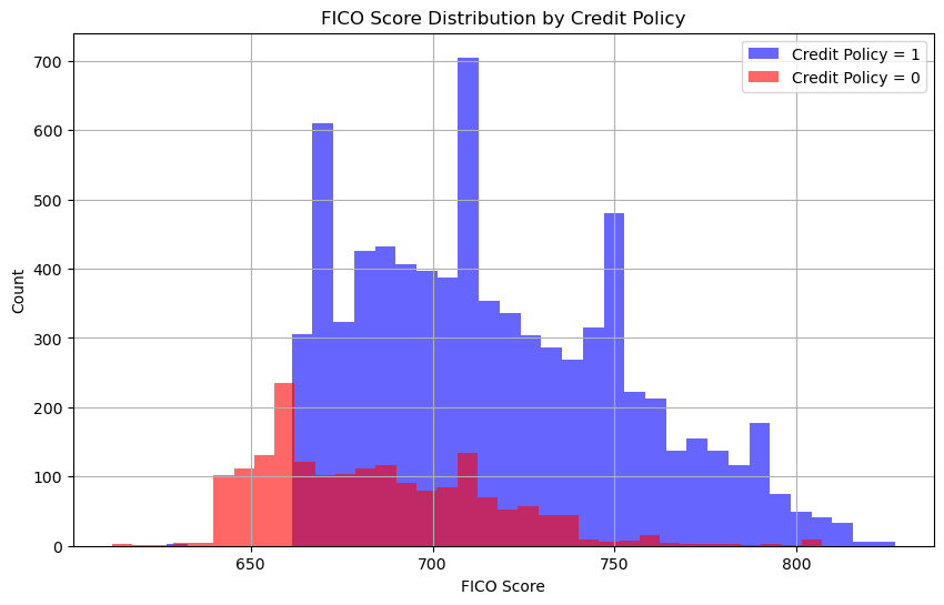
Insights: Borrowers with credit_policy = 1 (meeting the underwriting criteria) tend to have higher FICO scores, while those with credit_policy = 0 often have scores below 660.

Loan Repayment Status by FICO Score

Next, we examine how the FICO score relates to the not_fully_paid column:

# Histogram for FICO scores and repayment status
plt.figure(figsize=(10, 6))
loans[loans['not.fully.paid'] == 1]['fico'].hist(bins=35, alpha=0.6, label='Not Fully Paid = 1', color='red')
loans[loans['not.fully.paid'] == 0]['fico'].hist(bins=35, alpha=0.6, label='Not Fully Paid = 0', color='green')

plt.xlabel('FICO Score')
plt.ylabel('Count')
plt.legend()
plt.title('FICO Score Distribution by Loan Repayment Status')
plt.show()

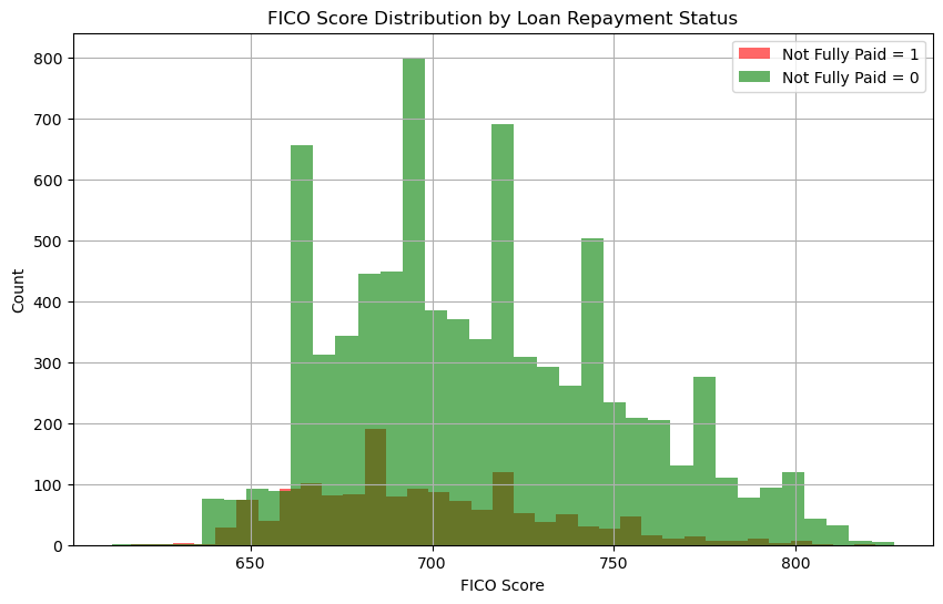
Insights: Most loans are fully repaid (not_fully_paid = 0), with a relatively uniform FICO score distribution across both categories.

Loan Purpose and Repayment Status

Using a count plot, we explore how loan purposes vary by repayment status:

import seaborn as sns

# Count plot for loan purpose
plt.figure(figsize=(11, 7))
sns.countplot(x='purpose', hue='not_fully_paid', data=loans, palette='Set1')

plt.xticks(rotation=45)
plt.title('Loan Purpose vs Repayment Status')
plt.show()

Insights: The most common loan purposes are debt consolidation and credit card refinancing. Across all purposes, the ratio of fully repaid to not fully paid loans remains consistent.

Relationship Between FICO Score and Interest Rate

We use a joint plot to visualize the correlation between the borrower’s FICO score and their interest rate (int_rate):

# Joint plot for FICO score vs. interest rate
sns.scatterplot(x='fico', y='int.rate', data=loans, hue='not.fully.paid')
plt.legend(bbox_to_anchor=(1.05, 1), loc=2, borderaxespad=0.)

Insights: The plot shows a negative correlation between fico and int.rate, with higher credit scores corresponding to lower interest rates. The points for loans not fully repaid (not.fully.paid = 1, shown in orange) are evenly distributed across the plot, indicating no strong relationship between repayment status and the fico-int.rate relationship.

Linear Trends: FICO Score, Interest Rate, and Policy

Finally, we explore linear trends in interest rates while segmenting by credit_policy and not_fully_paid:

# Linear model plot with hue and column split
sns.lmplot(x='fico', y='int.rate', data=loans, hue='credit.policy', col='not.fully.paid', palette='Set1', height=5, aspect=1.2)

Insights: This plot illustrates the relationship between fico and int.rate, split by not.fully.paid (loan repayment status) and distinguished by credit.policy. Key insights include:

Negative Correlation: Across both repayment statuses (not.fully.paid = 0 and not.fully.paid = 1), there is a strong negative correlation between fico and int.rate. Borrowers with higher fico scores are offered lower interest rates, reflecting their stronger creditworthiness.
Credit Policy Impact: Borrowers meeting the credit policy (credit.policy = 1) consistently have lower interest rates than those who do not (credit.policy = 0). This is evident from the positioning of the blue regression line below the red line in both subplots.
FICO Threshold Around 680: A vertical separation of red and blue points around a fico score of ~660 indicates a likely underwriting rule. Borrowers with fico scores below 660 are predominantly classified as credit.policy = 0 (higher risk), while those above are classified as credit.policy = 1 (lower risk). This reflects Lending Club's probable use of a FICO score cutoff in their lending decisions.

Overall, the plot highlights the interplay between credit policy, interest rates, and repayment behaviour, showing that while interest rates and credit policy vary significantly by fico, repayment status (not.fully.paid) does not heavily alter these trends.

4. Data Preprocessing

Before building the models, we need to prepare the dataset by encoding categorical variables and splitting the data into training and testing sets.

Handling Categorical Features

The dataset includes a categorical feature, purpose, which specifies the reason for the loan (e.g., debt consolidation, credit card). To make this column suitable for machine learning models, we use one-hot encoding to convert it into dummy variables:

import pandas as pd

# Create dummy variables for the 'purpose' column
cat_feats = ['purpose']
final_data = pd.get_dummies(loans, columns=cat_feats, drop_first=True)

# Check the resulting dataset
final_data.info()

<class 'pandas.core.frame.DataFrame'>
RangeIndex: 9578 entries, 0 to 9577
Data columns (total 19 columns):
 #   Column                      Non-Null Count  Dtype  
---  ------                      --------------  -----  
 0   credit.policy               9578 non-null   int64  
 1   int.rate                    9578 non-null   float64
 2   installment                 9578 non-null   float64
 3   log.annual.inc              9578 non-null   float64
 4   dti                         9578 non-null   float64
 5   fico                        9578 non-null   int64  
 6   days.with.cr.line           9578 non-null   float64
 7   revol.bal                   9578 non-null   int64  
 8   revol.util                  9578 non-null   float64
 9   inq.last.6mths              9578 non-null   int64  
 10  delinq.2yrs                 9578 non-null   int64  
 11  pub.rec                     9578 non-null   int64  
 12  not.fully.paid              9578 non-null   int64  
 13  purpose_credit_card         9578 non-null   bool   
 14  purpose_debt_consolidation  9578 non-null   bool   
 15  purpose_educational         9578 non-null   bool   
 16  purpose_home_improvement    9578 non-null   bool   
 17  purpose_major_purchase      9578 non-null   bool   
 18  purpose_small_business      9578 non-null   bool   
dtypes: bool(6), float64(6), int64(7)
memory usage: 1.0 MB

This process creates new binary columns (e.g., purpose.credit_card, purpose.debt_consolidation), representing each category in purpose. The drop_first=True argument ensures we avoid multicollinearity by dropping one dummy column for each category.

Splitting the Data

Next, we split the dataset into features (X) and target (y). The target variable is not.fully.paid, which we aim to predict:

from sklearn.model_selection import train_test_split

# Define X (features) and y (target)
X = final_data.drop('not.fully.paid', axis=1)
y = final_data['not.fully.paid']

# Split into training and testing sets
X_train, X_test, y_train, y_test = train_test_split(X, y, test_size=0.3, random_state=101)

Here:

X contains all the features except not.fully.paid.
y contains the target variable (not.fully.paid).
train_test_split divides the data into 70% training and 30% testing sets, ensuring reproducibility with random_state=101.

By the end of preprocessing, the data is ready for model training and evaluation. This step ensures categorical features are correctly encoded and the data is properly split for supervised learning.

5. Building the Models

In this step, we train two machine learning models: a Decision Tree and a Random Forest. These models aim to predict whether a loan is not fully repaid (not.fully.paid).

Training a Decision Tree

We start by creating and training a Decision Tree Classifier:

from sklearn.tree import DecisionTreeClassifier
from sklearn.metrics import classification_report, confusion_matrix

# Initialize the Decision Tree Classifier
tree = DecisionTreeClassifier()

# Fit the model to the training data
tree.fit(X_train, y_train)

# Make predictions on the test set
predictions_tree = tree.predict(X_test)

# Evaluate the model
print("Decision Tree Classification Report:")
print(classification_report(y_test, predictions_tree))
print("Confusion Matrix:")
print(confusion_matrix(y_test, predictions_tree))

Decision Tree Classification Report:
              precision    recall  f1-score   support

           0       0.86      0.82      0.84      2431
           1       0.20      0.25      0.22       443

    accuracy                           0.73      2874
   macro avg       0.53      0.53      0.53      2874
weighted avg       0.76      0.73      0.74      2874

Confusion Matrix:
[[1986  445]
 [ 332  111]]

The Decision Tree model achieves an overall accuracy of 73%, primarily driven by strong performance on class 0 (fully repaid loans), with a precision of 86% and a recall of 82%. However, its performance on class 1 (not fully repaid loans) is weak, with a precision of 20% and a recall of 25%, indicating that it struggles to correctly identify loans that are not fully repaid. The imbalance in performance reflects the class imbalance in the dataset, as class 0 dominates.

The confusion matrix shows the model correctly predicts 1,986 instances of 0 but misclassifies 445 of them, while for class 1, it only identifies 111 correctly, misclassifying 332.

Overall, the model prioritizes accuracy for the majority class (0) at the expense of minority class (1) predictions.

Training a Random Forest

Next, we train a Random Forest Classifier, an ensemble model that combines multiple decision trees for better performance and generalization:

from sklearn.ensemble import RandomForestClassifier

# Initialize the Random Forest Classifier with 300 trees
rf = RandomForestClassifier(n_estimators=300)

# Fit the model to the training data
rf.fit(X_train, y_train)

# Make predictions on the test set
predictions_rf = rf.predict(X_test)

# Evaluate the model
print("Random Forest Classification Report:")
print(classification_report(y_test, predictions_rf))
print("Confusion Matrix:")
print(confusion_matrix(y_test, predictions_rf))

Random Forest Classification Report:
              precision    recall  f1-score   support

           0       0.85      1.00      0.92      2431
           1       0.42      0.02      0.03       443

    accuracy                           0.84      2874
   macro avg       0.63      0.51      0.48      2874
weighted avg       0.78      0.84      0.78      2874

Confusion Matrix:
[[2420   11]
 [ 435    8]]

The Random Forest model achieves a high overall accuracy of 84%, driven by excellent performance on the majority class (not.fully.paid = 0), with precision of 85%, recall of 100%, and F1-score of 92%. However, it performs poorly on the minority class (not.fully.paid = 1), with a precision of 42%, recall of 2%, and F1-score of 3%.

The confusion matrix shows that it correctly predicts 2,420 fully repaid loans but misclassifies almost all not fully repaid loans (435 out of 443). This highlights the model's bias toward the majority class, likely due to class imbalance in the dataset.

6. Comparing Model Performance

The Decision Tree and Random Forest models yield different strengths and weaknesses in predicting loan repayment. Here’s a comparison of their performance metrics:

Key Observations:

The Decision Tree achieves moderate overall accuracy (73%) and handles the minority class (not.fully.paid = 1) better, with a recall of 25% and an F1 score of 22%.
The Random Forest improves overall accuracy to 84%, excelling at predicting the majority class (not.fully.paid = 0) with a precision of 85% and recall of 100%. However, it struggles with the minority class, achieving only 2% recall and a very low F1 score of 3%.

Performance Metrics Table:

Confusion Matrix Comparison:

Summary:

The Decision Tree performs better at identifying loans that are not fully repaid (class 1), but sacrifices some accuracy for the majority class.
The Random Forest achieves higher overall accuracy and excels at predicting fully repaid loans (class 0), but fails to detect the minority class (class 1), as seen in its extremely low recall for class 1.

In short, the choice between the models depends on the business goal. If accurately identifying high-risk loans (class 1) is critical, the Decision Tree may be more useful. However, for overall accuracy and generalization, the Random Forest is a better choice. Further improvement might involve addressing the class imbalance through techniques like oversampling or cost-sensitive learning.

7. Conclusion and Next Steps

In this project, we explored the application of Decision Trees and Random Forests to predict loan repayment status using real-world data from Lending Club. Here’s a summary of our findings:

Model Comparison

The Decision Tree achieved moderate overall accuracy (73%) and performed better at identifying loans not fully repaid (not.fully.paid = 1), with a recall of 25%.
The Random Forest excelled in overall accuracy (84%) and identifying fully repaid loans (not.fully.paid = 0), with perfect recall for this class, but struggled with the minority class, achieving only 2% recall for not.fully.paid = 1.

Insights from Data

Borrowers with lower FICO scores and higher interest rates are more likely to fall into the not.fully.paid = 1 category, although the distribution of these instances is relatively even across the dataset.
The dataset is imbalanced, with fully repaid loans (not.fully.paid = 0) comprising 84% of the data.

Next Steps for Improvement

To enhance the model’s ability to detect risky loans (minority class), future improvements could include:

Addressing Class Imbalance:

Use stratified sampling during train-test splits to maintain the class distribution.
Apply oversampling techniques like SMOTE (Synthetic Minority Oversampling Technique) to generate synthetic examples for the minority class.
Experiment with undersampling the majority class to balance the dataset.

2. Optimizing Model Training:

Adjust the class_weight parameter in Scikit-learn models to penalize misclassification of the minority class (not.fully.paid = 1).
Perform hyperparameter tuning for both models to optimize performance metrics like recall and F1-score.

3. Feature Engineering:

Incorporate additional features that might improve predictions, such as external credit history or economic indicators.
Engineer new features from existing data, like creating interaction terms between fico and int.rate.

4. Alternative Models:

Experiment with other classification models, such as Gradient Boosting, XGBoost, or Neural Networks, to see if they perform better on this dataset.

By addressing these steps, we can create a more robust model to help financial institutions better assess loan risks and improve decision-making in lending practices.

Appendix

Code: https://github.com/Minhhoang2606/Python-for-Data-Science-and-Machine-Learning-Bootcamp/blob/master/15-Decision-Trees-and-Random-Forests/03-Decision%20Trees%20and%20Random%20Forest%20Project.ipynb

Data source: https://www.kaggle.com/datasets/braindeadcoder/lending-club-data

Predicting Loan Repayment with Decision Trees and Random Forests Using Lending Club Data

Table of contents