Forecasting HR Cost - Time Series Modeling

Introduction

Cost in an organization is always a significant concern, and the management always wants to predict the cost before deciding on a future course of action. This article focuses on predicting cost using different time series models. Different models are used for predicting cost, such as autoregressive, moving average, and autoregressive integrated moving average (ARIMA) techniques, which are explained with examples. These techniques are used for any time series data existing in the organization. However, the methods discussed in this article can be used to extract different information according to an organization's requirements from any dataset in the human resource department.

HR Cost

HR cost is a key component of HR accounting. HR costs are mainly incurred from expenses related to salary, incentives, reimbursements, insurance, and fixed and miscellaneous costs. This includes total sot per hired employee across an entire company, the total compensation per employee, the total recruitment expenditures for every new hire across a particular time frame, expenses on job boards to draw valuable conclusions, the salary of recruiters, funds required to establish an employer brand like attending recruiting events, content writing, designing posters, and videos, social media, cost for partnerships with universities and institutions, cost of external recruiting agencies, recruiting technology costs like video interviewing tools, coding assessment tools.

Cost optimization continues to be a critical concern for many HR leaders. However, the HR professional should use different metrics that can be useful for determining an accurate assessment of total cost. For example, the quality of hire can be determined by comparing cost per hire and long-term performance evaluation. Different measures that an organization can take to reduce cost include restructuring the service delivery mechanism, incorporating flexibility for ensuring targeted utilization of capacities, redesigning processes to balance service delivery efficiency and effectiveness, developing the existing capacities to optimize services, balancing elements of the rewards model for effective cost optimization; structuring the workforce to align short-term business needs with long-term value; and achieving cost optimization effects through thoughtful layoff planning and execution.

Measure and forecast costs based on previous values are essential for smooth organizational functioning and effective strategy formulation.

Time Series Modeling

Forecasting helps formulate strategies in various businesses and is a basic need for managerial decision-making. Managers have to make decisions in uncertainty without knowing what will happen. Different methods, including qualitative and quantitative models, can obtain forecasting. Quantitative models include time series models and causal models. Causal models are used when one variable is dependent on the values of other variables. Time series data provide essential information related to time, and time series models attempt to predict the forecast demand (future values) using the past demand values (historical data). A time series is a series of data points in which each data point is associated with a timestamp. They play a significant role in understanding many details on specific factors over time. For example, stock price at different points of time on a given day, amount of sales in a region to varying months of the year.

Time series analysis can be used in many business applications to forecast a quantity into the future and explain its historical patterns. The ARIMA model is commonly used for time series forecasting. Exponential smoothing models were based on the data's description of trend and seasonality. At the same time, ARIMA models describe the autocorrelations in the data. Notably, every model is nonstationary, while ARIMA models can be stationary. ARIMA models use historical information to make predictions, which is a basis for complex models. ARIMA models support either no exponential or linear exponential smoothing but not nonlinear exponential smoothing. ARIMA is like a linear regression equation where the predictors depend on some parameters of the ARIMA model.

ARIMA models are a class of statistical models for analyzing and forecasting time series data. They explicitly cater to a suite of standard structures in time series data and, as such, provide a simple yet powerful method for making skillful time series forecasts. ARIMA generalizes the more straightforward autoregressive moving average and adds integration.

HR Cost Data

The HRCost file helps us understand KNIME usage. This dataset can be downloaded from the “Data” folder on the KNIME Community Hub.

The Forecast HR Cost – Time Series Modeling workflow can be downloaded from the KNIME Community Hub.

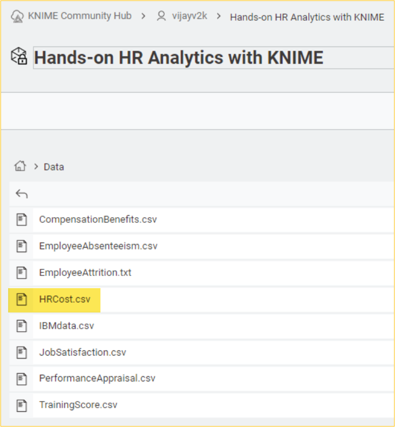
You are ready after downloading the CSV file from the Data folder.

Reading the CSV-based Dataset

The first step in our analysis will be to load the data for our exploratory analyses. We will do this first step using the CSV Reader node before we persist our analysis in a KNIME table.

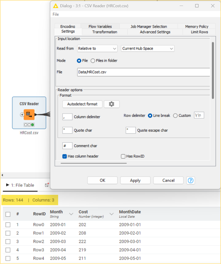
The KNIME table is created by loading the HRCost.csv CSV dataset. The above table shows that the employee dataset has 144 observations and 3 columns.

Filter / Subset observations for the HR Department

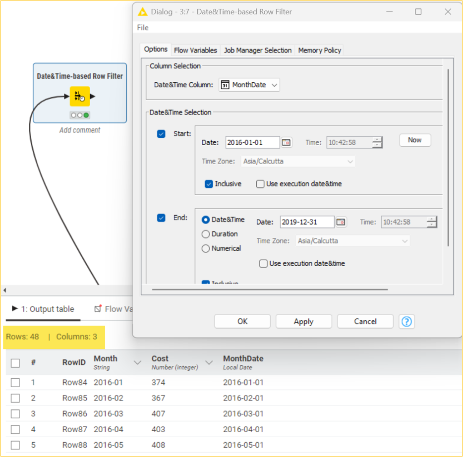
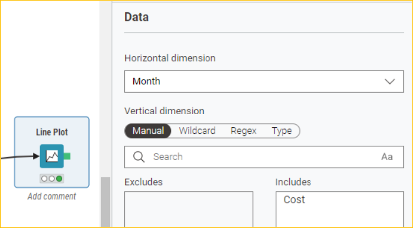
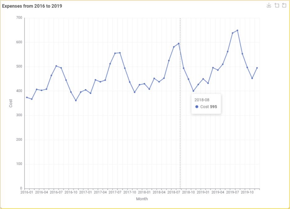
We will consider a subset of the dataset for our preliminary data exploration and visualization. Based on the MonthDate column, we can use the Date&TimeBased Row Filter node to filter out the Jan 2016 to Dec 2019 observations. After that, we will use the Line Plot node to display the monthly expenses from the Cost column in a line chart.

Testing Stationarity of Time Series Data

It is essential to check the stationarity of the series before doing forecasting. A time series is considered stationary if it does not have a trend or seasonal effects and this has consistent statistical properties over time. These properties include mean, variance, and autocovariance. Before applying statistical modeling methods, the time series is required in stationery. This is necessary for easy modeling and proper series forecasts because it should be the same if we take a specific behavior over time. Observations from a nonstationary time series show seasonal effects, trends, and other structures that depend on the time index. We can determine whether the tied series is stationary or nonstationary by looking at plots and checking trends or seasonality or by using statistical tests such as the Dickey-Fuller test.

We will use the statsmodels.tsa.stattools package in the Python Script node to apply the Dickey-Fuller test. The test's null hypothesis is that a unit root can represent the time series. This means that it is nonstationary and has some time-dependent structure. The alternative hypothesis (rejecting the null hypothesis) is that the time series is stationary. It suggests the time series does not have a unit root and does not have a time-dependent structure. We interpret this result using the p-value from the test. If the p-value is less than or equal to 0.05, it suggests we reject the null hypothesis. This means the data are stationary and do not have a unit root. If the p-value is more significant than 0.05, we fail to reject the null hypothesis, and the data have a unit root and are nonstationary. For practical analysis, it is also recommended that the rolling mean of the series be created and plotted.

import knime.scripting.io as knio

# Importing necessary libraries
from statsmodels.tsa.stattools import adfuller
import pandas as pd

# Load the input table as a pandas DataFrame
df = knio.input_tables[0].to_pandas()

# Ensure the series is extracted correctly
if "Cost" in df.columns:
    series = df["Cost"]
else:
    raise ValueError("The column 'Cost' is not found in the input table.")

# Applying Dickey-Fuller Test
# Null hypothesis: The time series is nonstationary
result = adfuller(series)

# Prepare the results of the Dickey-Fuller test
output_data = {
    "ADF Statistic": [result[0]],
    "p-value": [result[1]],
    "Critical Value 1%": [result[4]["1%"]],
    "Critical Value 5%": [result[4]["5%"]],
    "Critical Value 10%": [result[4]["10%"]]
}

# Convert the results to a pandas DataFrame
output_df = pd.DataFrame(output_data)

# Save the output DataFrame to the KNIME output table
knio.output_tables[0] = knio.Table.from_pandas(output_df)

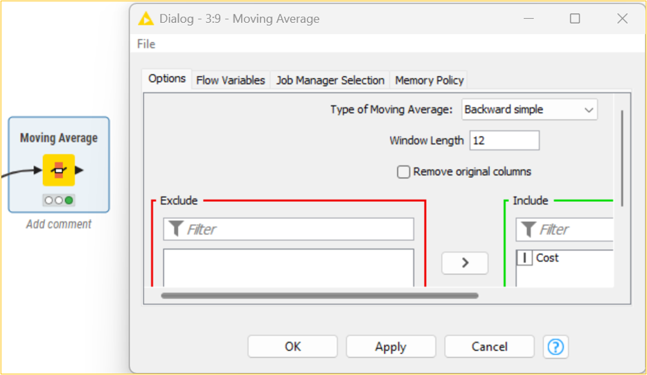
We will use the Moving Average node to create a backward simple moving average, with 12 windows, of the Cost column. Subsequently, we use the Line Plot node to plot the Cost and MA(Cost) columns.

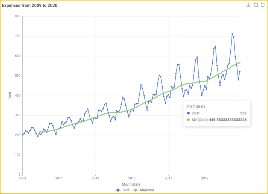
In our data, the p-value is 0.992, meaning the null hypothesis is accepted. This further implies that our series is nonstationary. This can be further interpreted by looking at the figure, which shows that the mean is increasing. It should be noted that for creating models, it is essential to make the series stationary before developing a model and doing forecasting.

Smoothing the Time Series Data

When the time series data have significant irregular components, we want a smooth curve to reduce these fluctuations. Curve smoothing is generally achieved using a simple moving average method, which is the best method to accomplish this using the Moving Average node. To roll the mean, we first take some (k) consecutive values and define a parameter k value. Generally, as the value of k increases, the plot becomes increasingly smoothed. The major challenge is to find the appropriate value of k that highlights the significant patterns in the data without under or over-smoothing. In our data, the value of k depends on the frequency. Since it is one year, we will consider the value of k as 12. For our Cost data, we will use natural logarithmic transformation using the ln() function of the Math Formula node to get the LnCost column because there is a strong positive trend. Subsequently, we use the Line Plot node to plot the LnCost and MA(LnCost) columns.

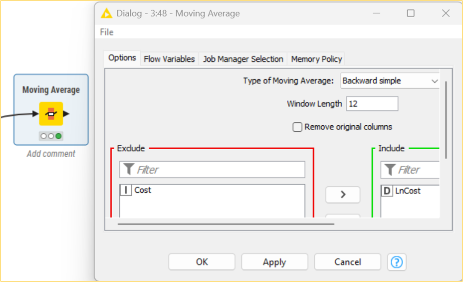
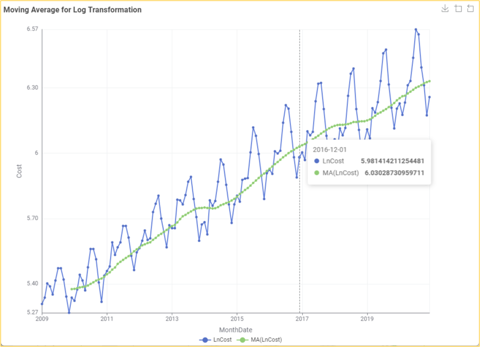
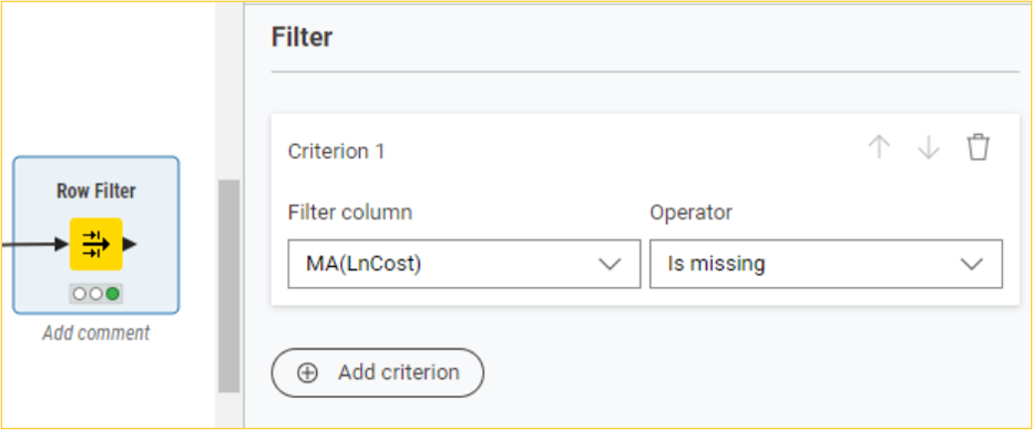
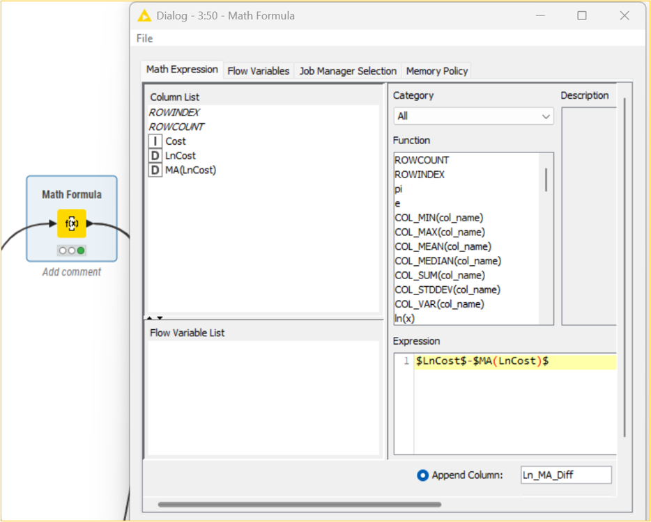
We can observe that the MA(LnCost) starts from Dec 2009. This is because we take the average of the last 12 values, and the rolling mean is not defined for the first 11 months. Thus, the first 11 months will have missing values. Since we cannot analyze missing values, dropping these rows using the Row Filter node is essential. Subsequently, we will find the difference between the two columns, LnCost and MA(LnCost), using the Math Formula node to create the Ln_MA_Diff column.

We will now determine the series' stationarity by performing the Dickey-Fuller test on the Ln_MA_Diff column and plotting its moving average series using the Line Plot node.

import knime.scripting.io as knio

# Importing necessary libraries
from statsmodels.tsa.stattools import adfuller
import pandas as pd

# Load the input table as a pandas DataFrame
df = knio.input_tables[0].to_pandas()

# Ensure the series is extracted correctly
if "Ln_MA_Diff" in df.columns:
    series = df["Ln_MA_Diff"]
else:
    raise ValueError("The column 'Ln_MA_Diff' is not found in the input table.")

# Applying Dickey-Fuller Test
# Null hypothesis: The time series is nonstationary
result = adfuller(series)

# Prepare the results of the Dickey-Fuller test
output_data = {
    "ADF Statistic": [result[0]],
    "p-value": [result[1]],
    "Critical Value 1%": [result[4]["1%"]],
    "Critical Value 5%": [result[4]["5%"]],
    "Critical Value 10%": [result[4]["10%"]]
}

# Convert the results to a pandas DataFrame
output_df = pd.DataFrame(output_data)

# Save the output DataFrame to the KNIME output table
knio.output_tables[0] = knio.Table.from_pandas(output_df)

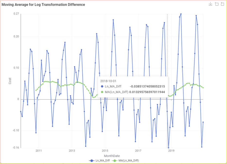
The p-value of 0.009 is less than 0.05. This means that the series is stationary at the 95% confidence interval. We can also observe from the visual representation that the rolling values vary slightly, but there is no specific trend. Hence, we can assume the series' stationarity. Thus, in the following sections, we will consider the data after the natural logarithmic transformation LnCost for developing the ARIMA model.

Forecast HR Cost Using Auto-Regressive (AR) Model

Objective: To forecast the HR cost using the Auto-Regressive (AR) model

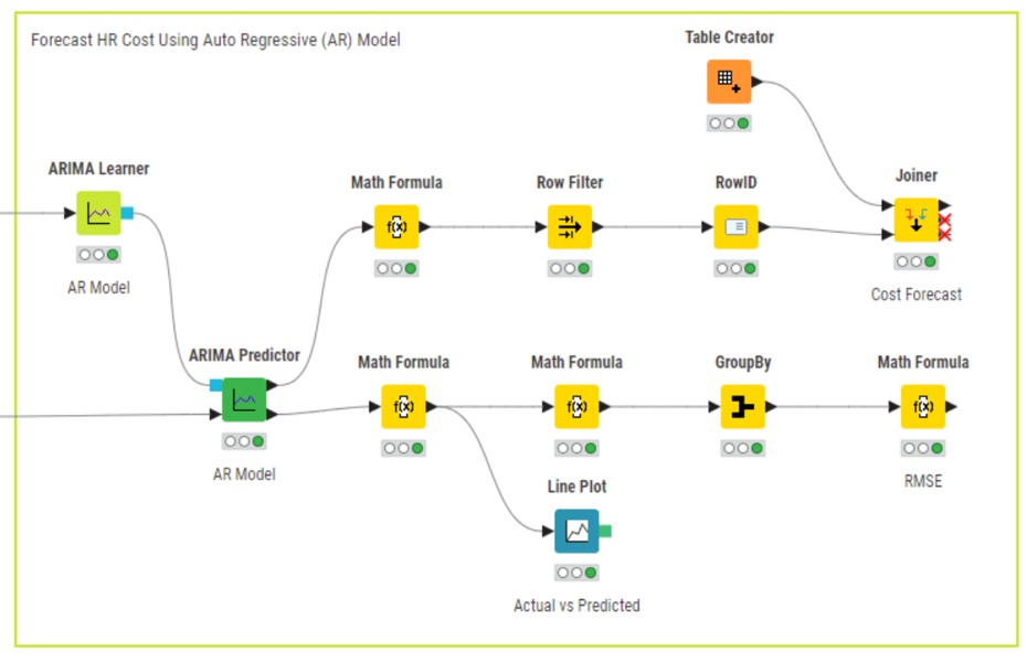
The AR model is created by considering the ARIMA function's third argument (moving average) to be zero. However, the value of the first argument denotes the lag value. For example, the ARIMA (5,1,0) creates an AR model, sets the lag value to 5 for autoregression, uses a difference order of 1 to make the time series stationary, and uses a moving average value of 0. Since the moving average component is 0, it can be considered as only an AR model.

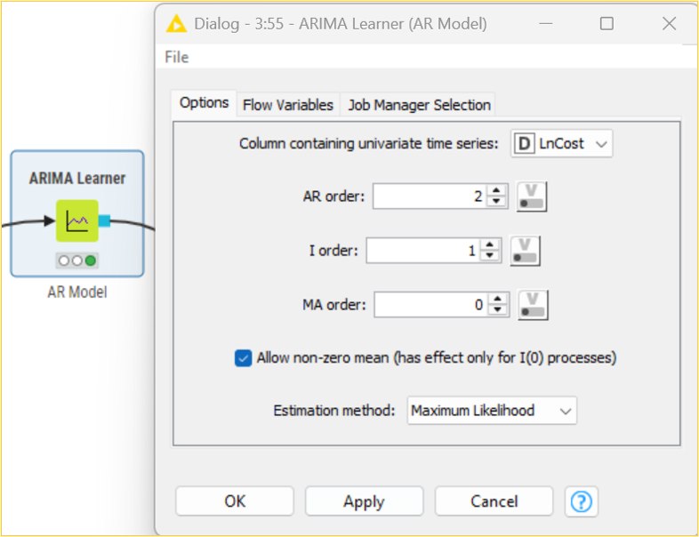
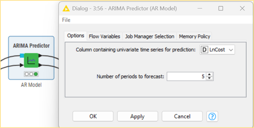
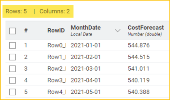
Using the maximum likelihood estimation method, we will use the ARIMA Learner node to develop an AR (2,1,0) model of lag two on the LnCost column. We will then use the ARIMA Predictor node to apply the regression model and obtain fitted values in the “In-sample predictions” output table. Based on this model, we can get the subsequent five-month forecasted cost CostForecast column by using the forecast option in the ARIMA Predictor node. The “Forecast” output shows the result in standard error and forecast values. Considering the forecasted values, the management of the organization can, thus, frame strategies and take decisions accordingly.

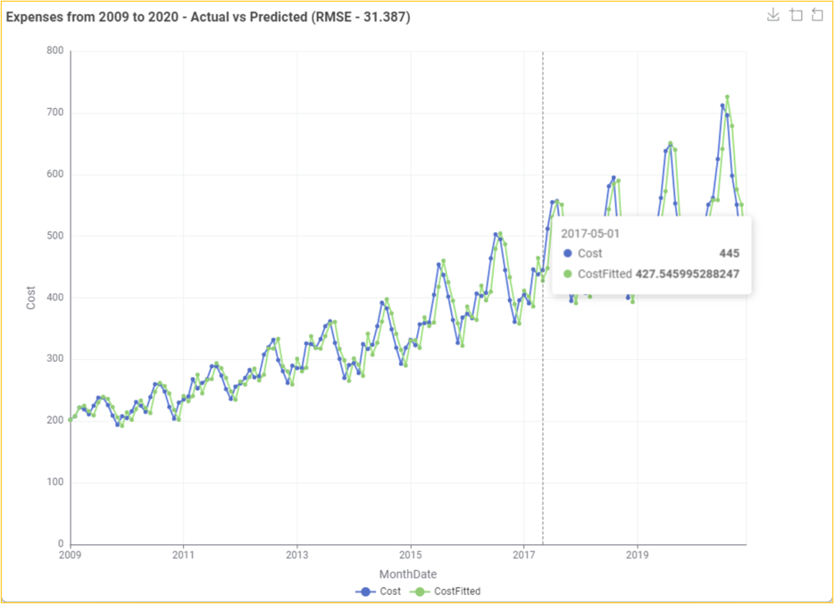
It should be noted that the fitted/forecast values need to be brought back to their original scale to predict actual values. The exp() function of the Math Formula node helps to determine the correct CostFitted values from the natural logarithmic LnCost(fitted values) values. It is essential to decide on the error of the developed model. This can be determined by observing the difference between the original and predicted values. The root mean squared function is one of the methods that can be used to determine the error (RMSE). Using multiple data manipulation nodes, the error in the developed AR model is 31.387. This means that there is a difference in the original and predicted values. It should be noted that the lower the value, the less the difference between the original and predicted values.

A visual display of the original Cost vs predicted CostFitted values uses the Line Plot node.

Forecast HR Cost Using Moving Average (MA) Model

Objective: To forecast the HR cost using the Moving Average (MA) model

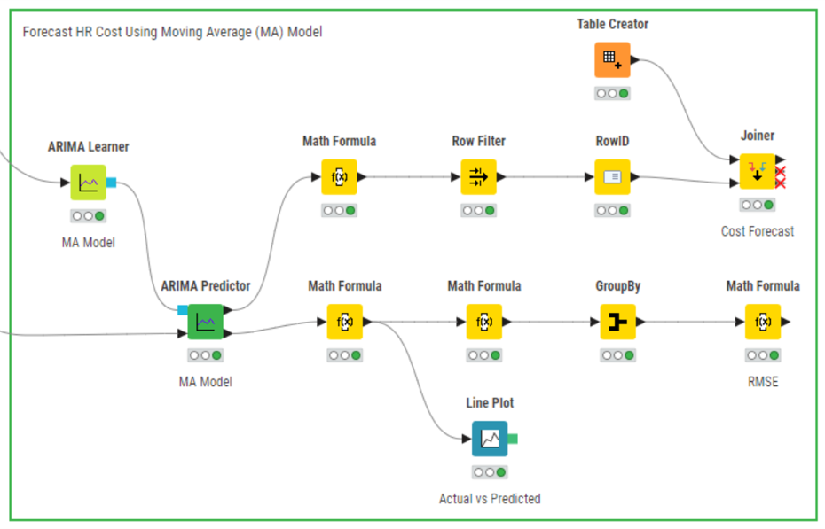
The MA model is created by considering the ARIMA function's first argument (autoregressive) to be zero. However, the value of the first argument denotes the lag value. For example, the ARIMA (0,1,3) creates an MA model and sets the lag value to 3 for the moving average, uses a difference order of 1 to make the time series stationary, and uses an autoregressive value of 0. Since the autoregressive component is 0, it can be considered as only an MA model.

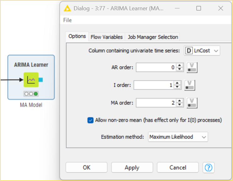
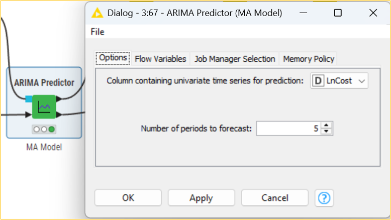
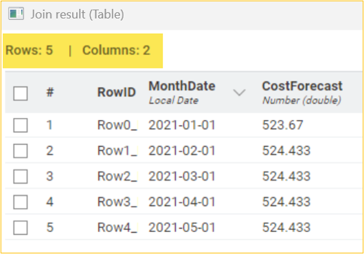
Using the maximum likelihood estimation method, we will use the ARIMA Learner node to develop an MA (0,1,2) on the LnCost column. We will then use the ARIMA Predictor node to apply the regression model and obtain fitted values in the “In-sample predictions” output table. Based on this model, we can get the subsequent five-month forecasted cost CostForecast column by using the forecast option in the ARIMA Predictor node. The “Forecast” output shows the result in standard error and forecast values. Considering the forecasted values, the management of the organization can, thus, frame strategies and take decisions accordingly.

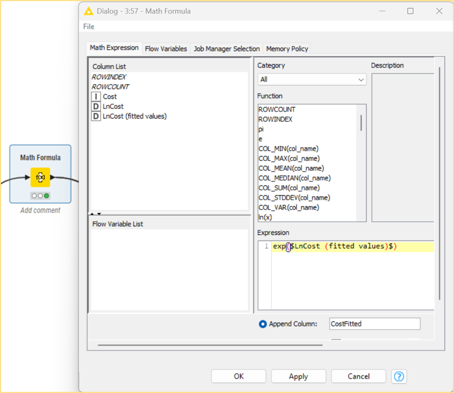
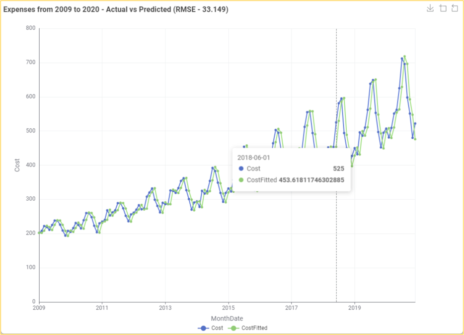
It should be noted that the fitted/forecast values need to be brought back to their original scale to predict actual values. The exp() function of the Math Formula node helps to determine the correct CostFitted values from the natural logarithmic LnCost(fitted values) values. It is essential to decide on the error of the developed model. This can be determined by observing the difference between the original and predicted values. The root mean squared function is one of the methods that can be used to determine the error (RMSE). Using multiple data manipulation nodes, the error in the developed AR model is 33.149. This means that there is a difference in the original and predicted values. It should be noted that the lower the value, the less the difference between the original and predicted values.

A visual display of the original Cost vs predicted CostFitted values uses the Line Plot node.

Forecast HR Cost Using ARIMA Model

Objective: To forecast the HR cost using the ARIMA model.

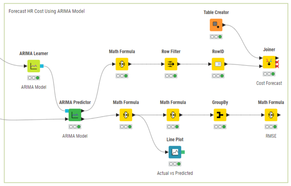
The ARIMA model is created by considering the first and third arguments as nonzero. For example, the ARIMA (3,1,3) creates an ARIMA model, sets the lag value to 3, and uses a difference order of 1 to make the time series stationary.

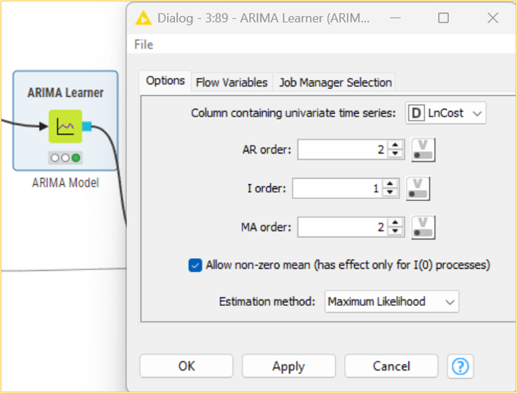
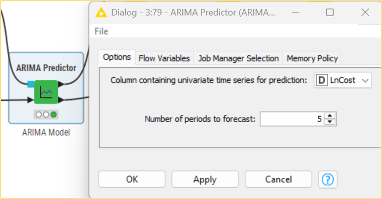
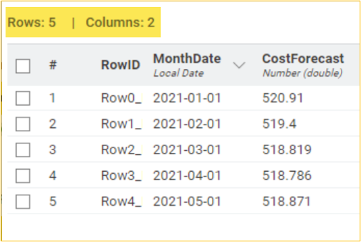
Using the maximum likelihood estimation method, we will use the ARIMA Learner node to develop an ARIMA (2,1,2) on the LnCost column. We will then use the ARIMA Predictor node to apply the regression model and obtain fitted values in the “In-sample predictions” output table. Based on this model, we can get the subsequent five-month forecasted cost CostForecast column by using the forecast option in the ARIMA Predictor node. The “Forecast” output shows the result in standard error and forecast values. Considering the forecasted values, the management of the organization can, thus, frame strategies and take decisions accordingly.

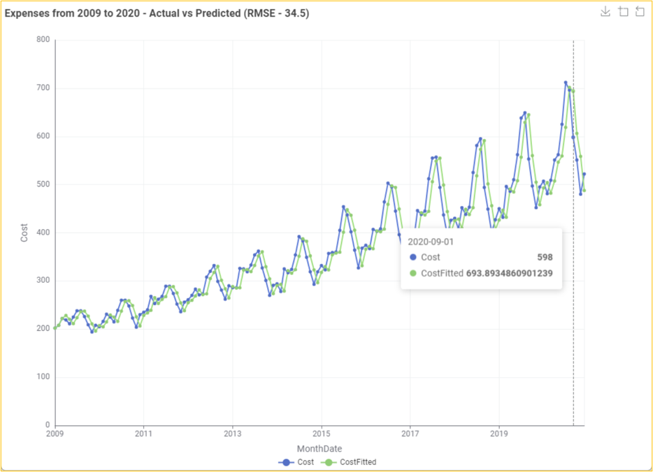
It should be noted that the fitted/forecast values need to be brought back to their original scale to predict actual values. The exp() function of the Math Formula node helps to determine the correct CostFitted values from the natural logarithmic LnCost(fitted values) values. It is essential to decide on the error of the developed model. This can be determined by observing the difference between the original and predicted values. The root mean squared function is one of the methods that can be used to determine the error (RMSE). Using multiple data manipulation nodes, the error in the developed AR model is 34.5. This means that there is a difference in the original and predicted values. It should be noted that the lower the value, the less the difference between the original and predicted values.

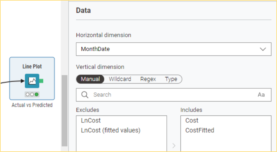
A visual display of the original Cost vs predicted CostFitted values uses the Line Plot node.

Summary

In conclusion, forecasting HR costs using time series modeling is valuable for organizations aiming to optimize their financial planning and decision-making processes. By employing models such as autoregressive (AR), moving average (MA), and autoregressive integrated moving average (ARIMA), organizations can effectively predict future HR expenses based on historical data. This enables management to make informed strategic decisions, align resources with business objectives, and implement cost-saving measures. The process involves ensuring data stationarity, applying appropriate smoothing techniques, and selecting the best-fitting model to achieve accurate forecasts. Ultimately, these predictive insights contribute to more efficient HR operations and overall organizational success.