Dimensional Modelling: A beginner's take
 Rutvik Joshi
This article is based on my learning and the content from Zach Wilson’s Data Engineering YouTube bootcamp.
TLDR;
Dimensional modeling involves organizing data into dimensions and measures, where dimensions answer "who" and "what" questions, and measures answer "how much" and "how many." The choice of data processing models, such as OLTP, OLAP, and master data, depends on the end-user's needs, ranging from analysts to non-tech users. Effective dimensional modeling requires understanding key business processes, end-user requirements, and handling slowly changing dimensions.
What is a dimension and a measure?
Dimensions are the attributes of an entity while Measures are the quantitative expression of the entity. In simple, dimensions provide the answers to who, what questions while measures provide answers to how much, in how many.
A good case is of a company:
| Dimensions | Measures |
| Company name (ABC) | Net Profit |
| Company type(Inc., partnership, limited…) | Total Sales |
| Products… | Quantity purchased |
A side note - Dimensions are of two types - Slowly changing || Fixed
What and for whom are you solving for?
Before you start modelling, identify who you are providing the data to, who is going to require that data to be processed so finely by your “esteemed” skills.
Is it an Analyst, Data Engineer or someone more nerdy like a ML Engineer or… a non-tech?
Below is a quick reference table to identify “who” and “what” they require.
| Factor / User | Analyst | Data Engineer | ML Engineer | Non - tech |
| Data Processing Models | Analytical Datasets OLAP | Master Datasets | OLAP - Identifiers and Numerical features | OLTP - Easy to read & direct |
| Query complexity | Easy | Tough | Easy → to Mid | NULL |
| Data Complexity | Low / Usually Simple (Decimal, string…) | High (Nested, array, struct) | Depends on the model being trained | Very Low - Patterns, Annotations, Charts |
OLTP | Master | OLAP data processing models
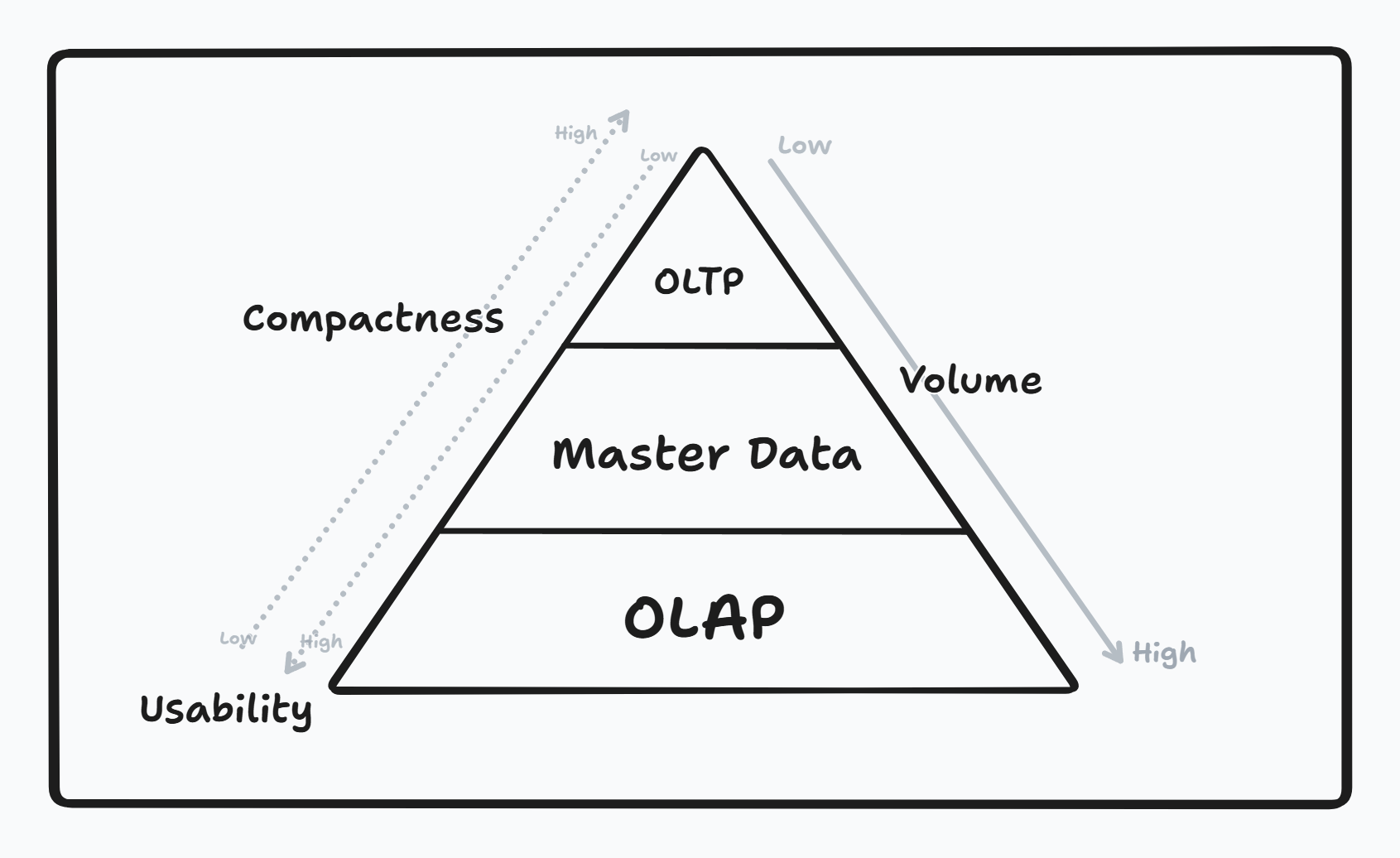
Based on the end user, data processing models can be categorized into a hierarchical level. Given an example of software engineer who works with the client side layer will often require Low latency/volume and High compact data since it is very specific and niche to the users who will be interacting with the application.
A good way to visualize the layers would be a pyramid structure with OLTP at the top and OLAP (which has entire data population or population subset) at the bottom as shared below.

To minimize the tradeoff between the OLTP and OLAP, master data is introduced which plays a critical role in:
The optimization for completeness of entity, the reduction in deduplication.
The use of ARRAY, MAP, STRUCT to further increase the compactness from OLAP layer.
To answer the question that arises, how can one develop master data tables which sit between the OLAP and OLTP models?
Depending on the data, a few ways that can help:
Cumulative Table Design
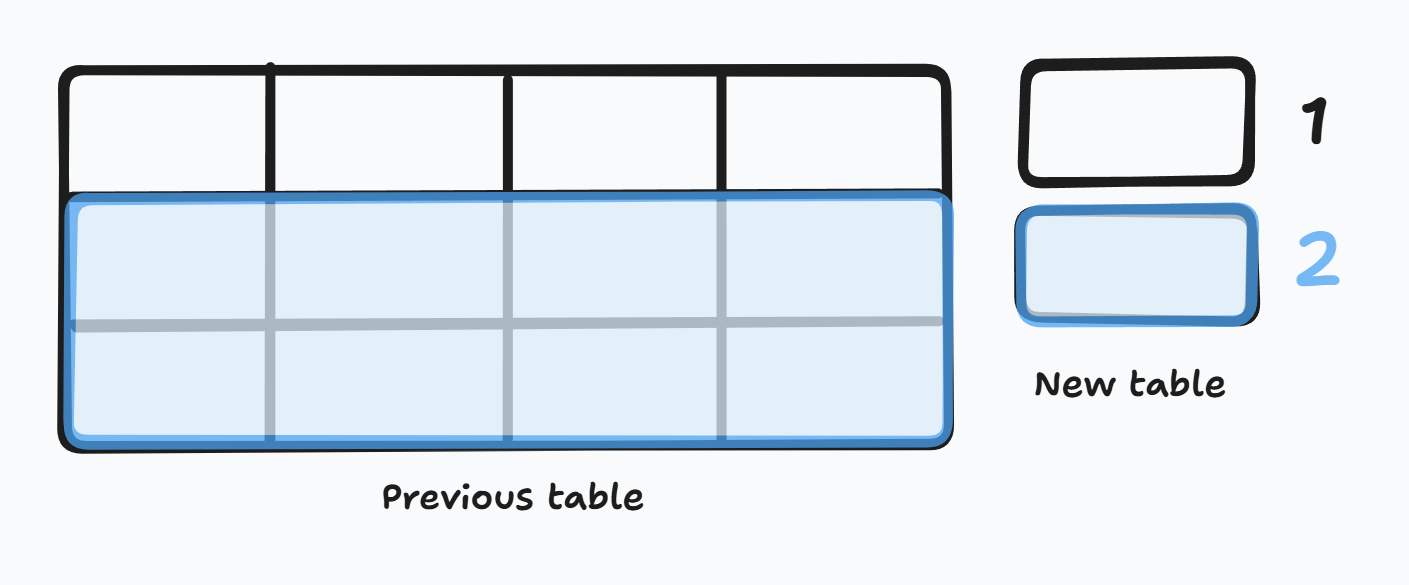
Based on a 2 table method where “yesterday” and “today” tables are cumulated to cover the entire scope of the dimensions for the dataset. Following steps are performed on the tables:
A FULL OUTER JOIN (betw. yesterday and today)
COALESCE of ids & unchanging dimensions
Computing cumulation metrics
Combining into arrays & changing values
-- Example query performed in Lab 1 - Sourced from https://github.com/DataExpert-io/data-engineer-handbook/blob/main/bootcamp/materials/1-dimensional-data-modeling/lecture-lab/pipeline_query.sql

WITH last_season AS ( -- Yesterday/previous season table
    SELECT * FROM players
    WHERE current_season = 1997

), this_season AS ( -- Today/this year table
     SELECT * FROM player_seasons
    WHERE season = 1998
)
INSERT INTO players
SELECT -- COALESCE of ids
        COALESCE(ls.player_name, ts.player_name) as player_name,
        COALESCE(ls.height, ts.height) as height,
        COALESCE(ls.college, ts.college) as college,
        COALESCE(ls.country, ts.country) as country,
        COALESCE(ls.draft_year, ts.draft_year) as draft_year,
        COALESCE(ls.draft_round, ts.draft_round) as draft_round,
        COALESCE(ls.draft_number, ts.draft_number)
            as draft_number,
        COALESCE(ls.seasons,
            ARRAY[]::season_stats[] -- Computed values
            ) || CASE WHEN ts.season IS NOT NULL THEN
                ARRAY[ROW(
                ts.season,
                ts.pts,
                ts.ast,
                ts.reb, ts.weight)::season_stats]
                ELSE ARRAY[]::season_stats[] END
            as seasons,
         CASE
             WHEN ts.season IS NOT NULL THEN --Combining into arrays and changing values
                 (CASE WHEN ts.pts > 20 THEN 'star'
                    WHEN ts.pts > 15 THEN 'good'
                    WHEN ts.pts > 10 THEN 'average'
                    ELSE 'bad' END)::scoring_class
             ELSE ls.scoring_class
         END as scoring_class,
         ts.season IS NOT NULL as is_active,
         1998 AS current_season

    FROM last_season ls
    FULL OUTER JOIN this_season ts -- FULL OUTER JOIN on the tables
    ON ls.player_name = ts.player_name
For Slowly Changing Dimensions:
Care for Idempotency (the ability of a data pipeline to produce same results in backfill or production, irrespective of the count of run or timestamp)
Care for achieving Type 2 Idempotency (mostly)
- Type 2 looks at a window time frame, allowing to track everything between the two dates (hence maintaining idempotency). You can learn more about the other types here.
Run length Encoding compression
Bring in the count-value pair compression indicating how many times the element repeats itself in the same pattern in the table.

Questions to ask?
Use these follow ups as pointers before you begin your dimensional modelling the next time:
What are the key business processes that need to be analyzed?
Who are the end-users of the data, and what are their specific requirements?
How will slowly changing dimensions be handled, and what type of changes are expected?
I appreciate your time reading through this. In the next article, I’ll share my learnings on Fact Modelling. Stay curious!
Subscribe to my newsletter
Read articles from Rutvik Joshi directly inside your inbox. Subscribe to the newsletter, and don't miss out.
Written by

Rutvik Joshi
Rutvik Joshi
I seek to create experiences. Currently doing it with, data, design and a blend of analytics.