How does PostgreSQL query planner work?
 Driptaroop Das
Introduction
We already know that postgres is a pretty solid RDMBS. It has consistently pretty good performance in queries. But how does it do that? How does it know which query plan to use? This is where the query planner comes in. We have already went through how postgres explain works in the past. Now we will go through how the query planner works in high level.
What is query planner?
The query planner is a part of the postgres that decides how to execute a query. It is responsible for deciding which query plan to use. It is a cost based optimizer. It uses the cost of the query plan to decide which query plan to use. The query planner is responsible for deciding how to execute a query, which indexes to use, which join to use, which scan to use etc.
But, a simple select query plan should be easy right? Just scan the table and return the rows. Use the index if it is there.
Well not exactly. Scanning the entire table is not always the best option. If the table is large or the filtered resultset is very small, scanning the entire table can be very slow. On the other hand, if the table is small or the filtered resultset contains a large percentage of the table rows, scanning the entire table can be faster than using the index.
Let's take an example.
Let's create a temporary table from pg_class table and create an index on it. (inspired from this excellent talk by Bruce Momjian) This table will get all the object names from pg_class table and create a temporary table with the first letter of the object name.
CREATE TEMPORARY TABLE sample (letter, junk) AS
SELECT substring(relname, 1, 1), repeat('x', 250)
FROM pg_class
ORDER BY random(); -- add rows in random order

CREATE INDEX i_sample on sample (letter);
What is a temporary table? A temporary table is a table that is created for the duration of a session. It is automatically dropped when the session ends.
We're going to run select letter from sample where letter = '<something>' on this table multiple times, so lets just create a function to do that.
CREATE OR REPLACE FUNCTION lookup_letter(text) RETURNS SETOF text AS
$$
BEGIN
    RETURN QUERY EXECUTE '
EXPLAIN SELECT letter
FROM sample
WHERE letter = ''' || $1 || '''';
END
$$ LANGUAGE plpgsql;
So right now, calling lookup_letter('p') will return the query plan for SELECT letter FROM sample WHERE letter = 'p'. Let's do that.
querying with the letter 'p':
select lookup_letter('p');
The result:
Bitmap Heap Scan on sample  (cost=4.16..10.07 rows=2 width=32)
  Recheck Cond: (letter = 'p'::text)
  ->  Bitmap Index Scan on i_sample  (cost=0.00..4.16 rows=2 width=0)
        Index Cond: (letter = 'p'::text)
Let's do a couple more.
querying with the letter 't':
select lookup_letter('t');
The result:
Bitmap Heap Scan on sample  (cost=4.16..10.07 rows=2 width=32)
  Recheck Cond: (letter = 't'::text)
  ->  Bitmap Index Scan on i_sample  (cost=0.00..4.16 rows=2 width=0)
        Index Cond: (letter = 't'::text)
querying with the letter 'i':
select lookup_letter('i');
Bitmap Heap Scan on sample  (cost=4.16..10.07 rows=2 width=32)
  Recheck Cond: (letter = 'i'::text)
  ->  Bitmap Index Scan on i_sample  (cost=0.00..4.16 rows=2 width=0)
        Index Cond: (letter = 'i'::text)
We can see that the query planner is always using the bitmap index scan (along with the heap scan) to get the rows. We can even showcase this by running the query for every value of letter in the sample table.
WITH letter (letter, count) AS (SELECT letter, COUNT(*)
                                FROM sample
                                GROUP BY 1)
SELECT letter    AS l,
       (SELECT *
        FROM lookup_letter(letter) AS l2
        LIMIT 1) AS lookup_letter
FROM letter;
the results:
| l | lookup_letter |
| _ | Bitmap Heap Scan on sample (cost=4.16..10.07 rows=2 width=32) |
| r | Bitmap Heap Scan on sample (cost=4.16..10.07 rows=2 width=32) |
| v | Bitmap Heap Scan on sample (cost=4.16..10.07 rows=2 width=32) |
| d | Bitmap Heap Scan on sample (cost=4.16..10.07 rows=2 width=32) |
| a | Bitmap Heap Scan on sample (cost=4.16..10.07 rows=2 width=32) |
| i | Bitmap Heap Scan on sample (cost=4.16..10.07 rows=2 width=32) |
| k | Bitmap Heap Scan on sample (cost=4.16..10.07 rows=2 width=32) |
| u | Bitmap Heap Scan on sample (cost=4.16..10.07 rows=2 width=32) |
| c | Bitmap Heap Scan on sample (cost=4.16..10.07 rows=2 width=32) |
| t | Bitmap Heap Scan on sample (cost=4.16..10.07 rows=2 width=32) |
| s | Bitmap Heap Scan on sample (cost=4.16..10.07 rows=2 width=32) |
| m | Bitmap Heap Scan on sample (cost=4.16..10.07 rows=2 width=32) |
| f | Bitmap Heap Scan on sample (cost=4.16..10.07 rows=2 width=32) |
| e | Bitmap Heap Scan on sample (cost=4.16..10.07 rows=2 width=32) |
| p | Bitmap Heap Scan on sample (cost=4.16..10.07 rows=2 width=32) |
We truncated the query plan until the end of first line so it can fit the table. But we can see for every letter, the query planner is using the bitmap index scan (along with the heap scan) to get the rows. So our index is getting used (Although for some unknown reason, the cost is always the same and its using bitmap index scan in place of normal index scan). Why is that?
Remember that we used a temporary table. There was a reason for that. That is autovacuum cannot ANALYZE (or VACUUM) temporary tables because these tables are only visible to the creating session.
Let's fill in the shoes of the autovaucum and analyze the table ourselves.
ANALYZE sample;
Running queries again on the analyzed table
Now let's run the queries again.
querying with the letter 'p':
select lookup_letter('p');
The result:
Seq Scan on sample  (cost=0.00..21.40 rows=357 width=2)
  Filter: (letter = 'p'::text)
querying with the letter 't':
select lookup_letter('t');
The result:
Bitmap Heap Scan on sample  (cost=4.20..17.27 rows=7 width=2)
  Recheck Cond: (letter = 't'::text)
  ->  Bitmap Index Scan on i_sample  (cost=0.00..4.20 rows=7 width=0)
        Index Cond: (letter = 't'::text)
querying with the letter 'i':
select lookup_letter('i');
Index Only Scan using i_sample on sample  (cost=0.15..11.98 rows=3 width=2)
  Index Cond: (letter = 'i'::text)
Welp! its all different now. The query planner is now using the seq scan for the letter 'p' and index only scan for the letter 'i'. The letter 't' is still using the bitmap index scan. In fact, we can query again for every letter in the sample table and see the query plan to verify the change in the planner behaviour.
WITH letter (letter, count) AS (SELECT letter, COUNT(*)
                                FROM sample
                                GROUP BY 1)
SELECT letter, count,
       (SELECT *
        FROM lookup_letter(letter) AS l2
        LIMIT 1) AS lookup_letter
FROM letter
ORDER BY 2 DESC;
The results:
| letter | count | lookup_letter |
| p | 357 | Seq Scan on sample (cost=0.00..21.40 rows=357 width=2) |
| c | 13 | Bitmap Heap Scan on sample (cost=4.25..20.69 rows=13 width=2) |
| r | 12 | Bitmap Heap Scan on sample (cost=4.24..20.14 rows=12 width=2) |
| t | 7 | Bitmap Heap Scan on sample (cost=4.20..17.27 rows=7 width=2) |
| f | 6 | Bitmap Heap Scan on sample (cost=4.19..17.25 rows=6 width=2) |
| s | 6 | Bitmap Heap Scan on sample (cost=4.19..17.25 rows=6 width=2) |
| _ | 5 | Index Only Scan using i_sample on sample (cost=0.15..15.79 rows=5 width=2) |
| u | 5 | Index Only Scan using i_sample on sample (cost=0.15..15.79 rows=5 width=2) |
| d | 4 | Index Only Scan using i_sample on sample (cost=0.15..13.88 rows=4 width=2) |
| v | 4 | Index Only Scan using i_sample on sample (cost=0.15..13.88 rows=4 width=2) |
| i | 3 | Index Only Scan using i_sample on sample (cost=0.15..11.98 rows=3 width=2) |
| m | 3 | Index Only Scan using i_sample on sample (cost=0.15..11.98 rows=3 width=2) |
| e | 3 | Index Only Scan using i_sample on sample (cost=0.15..11.98 rows=3 width=2) |
| a | 3 | Index Only Scan using i_sample on sample (cost=0.15..11.98 rows=3 width=2) |
| k | 1 | Index Only Scan using i_sample on sample (cost=0.15..8.17 rows=1 width=2) |
So we can see that the query planner is using a different query plan for different letters. This time I have included the count of the letters in the sample table as well. We can see that the query planner is using the seq scan for the letter 'p' which has the highest count in the table (the reason being lots of pg internal tables that starts with pg). The query planner is using the index only scan for the letters like 'i', 'm', 'e' etc. which have the lowest count in the table. The query planner is using the bitmap index scan for the letters 'c', 'r', 't', 'f' and 's' which have a moderate count in the table. So what happened? and why use seq scan at all if an index is there?
The answer is costs. But to understand that, we first have to understand what does ANALYZE do? and how the costs are calculated?
What does ANALYZE do?
ANALYZE is a command that collects statistics (more about it in the next section) about the tables and indexes in the database. It collects information about the distribution of the values in the columns, the number of rows in the table, the number of distinct values in the columns, etc. This information is used by the query planner to calculate the costs and to decide which query plan to use. The autovacuum daemon is a background process automatically that runs the analyze command on the tables and indexes in the database at regular intervals.
Statistics
Postgres statistics are the information about the distribution of the values in the columns, the number of rows in the table, the number of distinct values in the columns, etc. Postgres collects statistics about the tables and indexes in the database using the ANALYZE command. The statistics are stored in the pg_statistic table in the database.
Let's generate a table with some unevenly distributed data and check the statistics.
CREATE TABLE unequal_distribution (id SERIAL PRIMARY KEY, category TEXT);
INSERT INTO unequal_distribution (category) SELECT 'Common_Value_1' FROM generate_series(1, 50000);
INSERT INTO unequal_distribution (category) SELECT 'Occasional_Value_1' FROM generate_series(1, 20);
INSERT INTO unequal_distribution (category) SELECT 'Occasional_Value_2' FROM generate_series(1, 20);
INSERT INTO unequal_distribution (category) SELECT 'Occasional_Value_3' FROM generate_series(1, 20);
INSERT INTO unequal_distribution (category) SELECT 'Occasional_Value_4' FROM generate_series(1, 20);
INSERT INTO unequal_distribution (category) SELECT 'Occasional_Value_5' FROM generate_series(1, 20);
INSERT INTO unequal_distribution (category) SELECT 'Occasional_Value_6' FROM generate_series(1, 20);
INSERT INTO unequal_distribution (category) SELECT 'Occasional_Value_8' FROM generate_series(1, 20);
INSERT INTO unequal_distribution (category) SELECT 'Occasional_Value_9' FROM generate_series(1, 20);
INSERT INTO unequal_distribution (category) SELECT 'Occasional_Value_10' FROM generate_series(1, 20);
INSERT INTO unequal_distribution (category) SELECT 'Rare_Value_1' FROM generate_series(1, 5);
INSERT INTO unequal_distribution (category) SELECT 'Rare_Value_2' FROM generate_series(1, 5);
INSERT INTO unequal_distribution (category) SELECT 'Rare_Value_3' FROM generate_series(1, 5);
INSERT INTO unequal_distribution (category) SELECT 'Rare_Value_4' FROM generate_series(1, 5);
INSERT INTO unequal_distribution (category) SELECT 'Rare_Value_5' FROM generate_series(1, 5);
INSERT INTO unequal_distribution (category) SELECT 'Rare_Value_6' FROM generate_series(1, 5);
INSERT INTO unequal_distribution (category) SELECT 'Rare_Value_7' FROM generate_series(1, 5);
INSERT INTO unequal_distribution (category) SELECT 'Rare_Value_8' FROM generate_series(1, 5);
INSERT INTO unequal_distribution (category) SELECT 'Rare_Value_9' FROM generate_series(1, 5);
INSERT INTO unequal_distribution (category) SELECT 'Rare_Value_10' FROM generate_series(1, 5);
INSERT INTO unequal_distribution (category) SELECT 'Ultra_Rare_Value_1' FROM generate_series(1, 2);
INSERT INTO unequal_distribution (category) SELECT 'Ultra_Rare_Value_2' FROM generate_series(1, 2);
INSERT INTO unequal_distribution (category) SELECT 'Ultra_Rare_Value_3' FROM generate_series(1, 2);
INSERT INTO unequal_distribution (category) SELECT 'Ultra_Rare_Value_4' FROM generate_series(1, 2);
INSERT INTO unequal_distribution (category) SELECT 'Ultra_Rare_Value_5' FROM generate_series(1, 2);
INSERT INTO unequal_distribution (category) SELECT 'Ultra_Rare_Value_6' FROM generate_series(1, 2);
INSERT INTO unequal_distribution (category) SELECT 'Ultra_Rare_Value_7' FROM generate_series(1, 2);
INSERT INTO unequal_distribution (category) SELECT 'Ultra_Rare_Value_8' FROM generate_series(1, 2);
INSERT INTO unequal_distribution (category) SELECT 'Ultra_Rare_Value_9' FROM generate_series(1, 2);
INSERT INTO unequal_distribution (category) SELECT 'Ultra_Rare_Value_10' FROM generate_series(1, 2);
INSERT INTO unequal_distribution (category) SELECT null FROM generate_series(1, 100);
-- ANALYZE the table (although Auto vacuum should do this automatically)
ANALYZE unequal_distribution;
Now that the table is generated, lets check the statistics.
select * from pg_statistic where starelid = 'public.unequal_distribution'::regclass;
This will return a somewhat cryptic result from the pg_statistic table. It will look something like this:
| starelid | staattnum | stainherit | stanullfrac | stawidth | stadistinct | stakind1 | stakind2 | stakind3 | stakind4 | stakind5 | staop1 | staop2 | staop3 | staop4 | staop5 | stacoll1 | stacoll2 | stacoll3 | stacoll4 | stacoll5 | stanumbers1 | stanumbers2 | stanumbers3 | stanumbers4 | stanumbers5 | stavalues1 | stavalues2 | stavalues3 | stavalues4 | stavalues5 |
| 16673 | 1 | false | 0 | 4 | -1 | 2 | 3 | 0 | 0 | 0 | 97 | 97 | 0 | 0 | 0 | 0 | 0 | 0 | 0 | 0 | null | {1.00000000} | null | null | null | {3,512,1017,1521,1995,2497,2997,3495,4033,4523,5054,5563,6077,6574,7089,7586,8107,8611,9128,9639,10135,10644,11126,11629,12129,12594,13119,13593,14086,14595,15105,15651,16140,16675,17223,17706,18236,18742,19231,19728,20242,20756,21265,21749,22227,22747,23261,23760,24251,24751,25257,25777,26246,26748,27257,27750,28254,28748,29243,29745,30295,30819,31311,31855,32366,32879,33368,33870,34399,34879,35359,35883,36393,36898,37369,37874,38335,38815,39301,39813,40295,40788,41279,41777,42275,42763,43270,43793,44297,44826,45317,45786,46314,46851,47326,47829,48332,48835,49318,49831,50350} | null | null | null | null |
| 16673 | 2 | false | 0.0021666666 | 15 | 26 | 1 | 2 | 3 | 0 | 0 | 98 | 664 | 664 | 0 | 0 | 100 | 100 | 100 | 0 | 0 | {0.9933666586875916,0.0005333333392627537,0.00039999998989515007,0.00039999998989515007,0.000366666674381122,0.000366666674381122,0.000366666674381122,0.00033333332976326346,0.0003000000142492354,0.0003000000142492354} | null | {1.00000000} | null | null | {Common_Value_1,Occasional_Value_2,Occasional_Value_5,Occasional_Value_9,Occasional_Value_1,Occasional_Value_4,Occasional_Value_6,Occasional_Value_8,Occasional_Value_10,Occasional_Value_3} | {Rare_Value_1,Rare_Value_1,Rare_Value_10,Rare_Value_2,Rare_Value_2,Rare_Value_4,Rare_Value_6,Rare_Value_7,Rare_Value_7,Rare_Value_8,Rare_Value_9,Rare_Value_9,Ultra_Rare_Value_3,Ultra_Rare_Value_5,Ultra_Rare_Value_6,Ultra_Rare_Value_9} | null | null | null |
Postgres actually uses this information to calculate the costs of the query plan. But obviously, this table was never meant to be read by us mere mortals. So, postgres gracefully provides us with the pg_stats view to understand the statistics in a more human readable form.
Understanding pg_stats:
SELECT * FROM pg_stats WHERE tablename = 'unequal_distribution';
The pg_stats view will return a more readable result. It will look something like this:
| schemaname | tablename | attname | inherited | null_frac | avg_width | n_distinct | most_common_vals | most_common_freqs | histogram_bounds | correlation | most_common_elems | most_common_elem_freqs | elem_count_histogram | range_length_histogram | range_empty_frac | range_bounds_histogram |
| public | unequal_distribution | id | false | 0 | 4 | -1 | null | null | {3,512,1017,1521,1995,2497,2997,3495,4033,4523,5054,5563,6077,6574,7089,7586,8107,8611,9128,9639,10135,10644,11126,11629,12129,12594,13119,13593,14086,14595,15105,15651,16140,16675,17223,17706,18236,18742,19231,19728,20242,20756,21265,21749,22227,22747,23261,23760,24251,24751,25257,25777,26246,26748,27257,27750,28254,28748,29243,29745,30295,30819,31311,31855,32366,32879,33368,33870,34399,34879,35359,35883,36393,36898,37369,37874,38335,38815,39301,39813,40295,40788,41279,41777,42275,42763,43270,43793,44297,44826,45317,45786,46314,46851,47326,47829,48332,48835,49318,49831,50350} | 1 | null | null | null | null | null | null |
| public | unequal_distribution | category | false | 0.0021666666 | 15 | 26 | {Common_Value_1,Occasional_Value_2,Occasional_Value_5,Occasional_Value_9,Occasional_Value_1,Occasional_Value_4,Occasional_Value_6,Occasional_Value_8,Occasional_Value_10,Occasional_Value_3} | {0.9933666586875916,0.0005333333392627537,0.00039999998989515007,0.00039999998989515007,0.000366666674381122,0.000366666674381122,0.000366666674381122,0.00033333332976326346,0.0003000000142492354,0.0003000000142492354} | {Rare_Value_1,Rare_Value_1,Rare_Value_10,Rare_Value_2,Rare_Value_2,Rare_Value_4,Rare_Value_6,Rare_Value_7,Rare_Value_7,Rare_Value_8,Rare_Value_9,Rare_Value_9,Ultra_Rare_Value_3,Ultra_Rare_Value_5,Ultra_Rare_Value_6,Ultra_Rare_Value_9} | 1 | null | null | null | null | null | null |
Let's understand the columns in the pg_stats view:
schemaname: The schema name of the table.tablename: The name of the table. In this case, it isunequal_distribution.attname: The name of the column. We would be focusing on thecategorycolumn since it has the uneven distribution of values.inherited: Whether the column is inherited from a parent table.null_frac: The fraction of NULL values in the column. The range is from 0 to 1. A value of 0 means that there are no NULL values in the column. A value of 1 means that all the values in the column are NULL.avg_width: The average size of the values in the column. This is used to calculate the size of the rows in the table.n_distinct: the estimated number of distinct values in the column. If less than zero, the negative of the number of distinct values divided by the number of rows. (The negated form is used when ANALYZE believes that the number of distinct values is likely to increase as the table grows; the positive form is used when the column seems to have a fixed number of possible values.) For example, -1 indicates a unique column in which the number of distinct values is the same as the number of rows.most_common_vals: A list of the most common values in the column. (Null if no values seem to be more common than any others. This is an array. Values in this column will typically have low selectivity, i.e., they will match a large fraction of the rows.most_common_freqs: A list of the frequencies of the most common values, i.e., number of occurrences of each divided by total number of rows. This is an array and has the same number of elements as themost_common_valsarray presenting the frequency of the corresponding value. This is the selectivity of the value.histogram_bounds: A list of values that divide the column's values into groups of approximately equal population. The values in most_common_vals, if present, are omitted from this histogram calculation.correlation: Statistical correlation between physical row ordering and logical ordering of the column values. This ranges from -1 to +1. When the value is near -1 or +1, an index scan on the column will be estimated to be cheaper than when it is near zero, due to reduction of random access to the disk.
A more detailed definition of columns for pg_stats can be found here in documentation. We'll cover more about how statistics are gathered in a later post.
Calculating the query plan costs
Now since postgres has the statistics, it can calculate the costs of the query plan for all possible query plans and chooses the one with the lowest cost. For example, a simple select query like SELECT * FROM table WHERE column = 'value' can have multiple query plans. It can use one of three strategies for this query.
seq scan
index scan
bitmap index scan
Postgres calculates the cost of all these query plans and chooses the one with the lowest cost. The following is the example of how the costs are calculated for a seq scan.
Calculating the cost of a seq scan
Postgres uses the following formula for calculating the cost of a seq scan for a simple select * from unequal_distribution where category = 'Common_Value_1'; query:
seq scan cost = (disk pages read * seq_page_cost) + (rows scanned * cpu_tuple_cost) + [if there are filters] (then number of rows filter applied on * cpu_operator_cost)
disk pages read: The number of disk pages read from the table. Regardless of which values we are trying to get, we have to read all the pages of the table. This is the number of pages in the table. We can get the number of pages in the table using the following query:SELECT relpages FROM pg_class WHERE relname = 'unequal_distribution';which is 321 in our case. So,
disk pages readis 321.seq_page_cost: The cost of reading a page from the disk. This is a configuration parameter in postgres. The default value is 1.0.rows scanned: The number of rows scanned from the table. In seq scan we have to scan all the rows. This is the number of rows in the table. We can get the number of rows in the table using the following query:SELECT reltuples FROM pg_class WHERE relname = 'unequal_distribution';which is 50350 in our case. So,
rows scannedis 50350.cpu_tuple_cost: The cost of processing a tuple in the CPU. This is a configuration parameter in postgres. The default value is 0.01.cpu_operator_cost: The cost of applying a filter on a row. This is a configuration parameter in postgres. The default value is 0.0025.then number of rows filter applied on: Since we have to apply the where clause filter on all the rows, this is the number of rows in the table. This is 50350 in our case.
So, total cost is: (321 * 1.0) + (50350 * 0.01) + (50350 * 0.0025) = 950.375
We, can confirm it by running the query plan for the query:
explain select * from unequal_distribution where category = 'Common_Value_1';
The result:
Seq Scan on unequal_distribution  (cost=0.00..950.38 rows=50016 width=19)
  Filter: (category = 'Common_Value_1'::text)
Our calculations were correct. The cost of the seq scan is 950.38 ~= 950.375.
Cost of index scan
PostgreSQL does not use a single, closed‐form “one‐line” equation to estimate the cost of an index scan; rather, it combines several components (I/O cost for reading index pages, CPU cost for processing index entries, I/O cost for reading the matching table pages, and CPU cost for processing table rows). However, in most simplified explanations (and in the PostgreSQL source code’s costsize.c), the total cost of a basic index scan can be approximated by a formula of the form:
(startup cost) + (index pages * random_page_cost) + (index tuples * cpu_index_tuple_cost) + (heap pages * random_page_cost) + (heap tuples * cpu_tuple_cost)
This calculation is too complex to do in this post. So rather, we would force postgres to use the index scan and see the cost. In order for us to force postgres to use the index scan, we have to create an index, disable the seq scan and disable the bitmap scan. We can do this by running the following commands:
create index i_category on unequal_distribution (category);
set enable_seqscan = off;
set enable_indexscan = on;
set enable_bitmapscan = off;
Now lets try to execute the query again and try to figure out the cost from the query plan.
explain select * from unequal_distribution where category = 'Common_Value_1';
The result:
Index Scan using i_category on unequal_distribution  (cost=0.29..1381.53 rows=50014 width=19)
  Index Cond: (category = 'Common_Value_1'::text)
The cost is 1381.53. This is the cost of the index scan.
Cost of bitmap index scan
The cost of the bitmap index scan is calculated in a similar way to the index scan. The only difference is that the bitmap index scan works in two steps.
Bitmap Index Scan: builds an in‐memory bitmap of all TIDs (row locations) that match the index condition.
Bitmap Heap Scan: uses that bitmap to read the corresponding table pages (in sorted order of block number), then rechecks or returns the matching rows.
The total cost of the bitmap index scan is the sum of the costs of the two steps.
Total Cost=Cost(BitmapIndexScan)+Cost(BitmapHeapScan).

=> BitmapIndexScan = (index startup+index pages*random_page_cost+index tuples*(cpu_index_tuple_cost+cpu_operator_cost)
=> BitmapHeapScan = (heap startup+heap pages*effective_page_cost+heap tuples*cpu_tuple_cost)
Like the index scan it is also too complex to calculate in this post. We can force postgres to use the bitmap index scan and see the cost from the query plan.
set enable_seqscan = off;
set enable_indexscan = off;
set enable_bitmapscan = on;
Now lets try to execute the query again and try to figure out the cost from the query plan.
explain select * from unequal_distribution where category = 'Common_Value_1';
The result:
Bitmap Heap Scan on unequal_distribution  (cost=571.90..1518.07 rows=50014 width=19)
  Recheck Cond: (category = 'Common_Value_1'::text)
  ->  Bitmap Index Scan on i_category  (cost=0.00..559.39 rows=50014 width=0)
        Index Cond: (category = 'Common_Value_1'::text)
From this, we can see that the cost of the bitmap index scan is 1518.07. This is the cost of the bitmap index scan.
Lowest cost wins strategy
So far we have seen how the costs are calculated for the seq scan, index scan and bitmap index scan.
| Strategy | Cost |
| Seq Scan | 950.38 |
| Index Scan | 1381.53 |
| Bitmap Index Scan | 1518.07 |
The query planner will choose the strategy with the lowest cost. In this case, the seq scan has the lowest cost. So, the query planner will choose the seq scan strategy for the query. We can prove this but keeping the index intact but enabling all the strategies and running the query plan.
set enable_seqscan = on;
set enable_indexscan = on;
set enable_bitmapscan = on;
Now lets try to execute the query again and try to figure out the cost from the query plan.
explain select * from unequal_distribution where category = 'Common_Value_1';
The result:
Seq Scan on unequal_distribution  (cost=0.00..950.38 rows=50014 width=19)
  Filter: (category = 'Common_Value_1'::text)
The query planner is using the seq scan strategy for the query. This is because the seq scan has the lowest cost among all the strategies.
The same is not true for the rarer values though. For example, the example for selecting the value 'Ultra_Rare_Value_1' is:
explain select * from unequal_distribution where category = 'Ultra_Rare_Value_1';
The result is:
Index Scan using i_category on unequal_distribution  (cost=0.29..8.36 rows=4 width=19)
  Index Cond: (category = 'Ultra_Rare_Value_1'::text)
The cost for index scan here is 8.36.
For the seq scan the cost is similar to "Common_Value_1" which is 950.38. So, the query planner will choose the index scan strategy for the query because it has the lowest cost.
Why is the index scan cost lower than the seq scan cost for the rarer values?
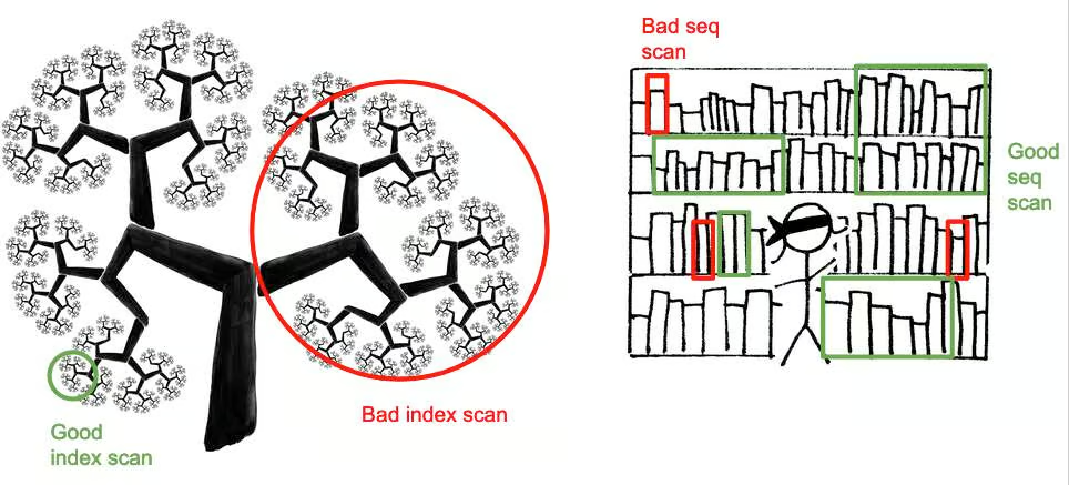
It may be interesting to note why the index scan cost is lower than the seq scan cost for the rarer values (high selectivity). This is because the index scan only has to read the index pages and the heap pages for the matching rows. The seq scan has to read all the pages of the table. So, the index scan is faster than the seq scan for the rarer values. An intuitive way to understand this would be to think an index like a tree. It's fast to find one item traversing through a tree, which is the "index scan". But finding a lot of items involves running through the tree over and over and over. It is slow to index scan all the records in a tree.
On the other hand, the seq scan is faster than the index scan for the common values (low selectivity) because the index scan has to read the index pages and then fetch the corresponding heap pages for the matching rows. These pages are read in random disk reads. The seq scan reads the pages in sequential disk reads. The sequential disk reads are much faster than the random disk reads. So, with large enough datasets, the seq scan is faster than the index scan for the common values. An intuitive way to understand this would be to think rows are books in a very large bookshelf store sequentially. It is time-consuming to find a small subset of books from that row of a large number of books. But if you have to pull down almost all the books from the row, it is faster to just go through them and pull down as necessary.
This awesome picture from this blog post really explains it well:
Conclusion
In this post we have seen how the query planner uses the statistics to calculate the costs of the query plans and chooses the one with the lowest cost. We have seen how the costs are calculated for the seq scan. We have also seen how we can force the query planner to use a particular strategy (like index scan or bitmap index scan) by enabling or disabling the strategies. In the next post, we will see how the statistics are gathered and how can we influence them.
References
- https://momjian.us/main/writings/pgsql/optimizer.pdf
- https://www.crunchydata.com/blog/indexes-selectivity-and-statistics
- https://www.postgresql.org/docs/current/indexes-selectivity.html
- https://www.postgresql.org/docs/current/index-cost-estimation.html
- https://www.postgresql.org/docs/current/using-explain.html
- https://github.com/postgres/postgres/blob/master/src/backend/optimizer/path/costsize.c
- https://github.com/postgres/postgres/blob/master/src/backend/utils/adt/selfuncs.c
Subscribe to my newsletter
Read articles from Driptaroop Das directly inside your inbox. Subscribe to the newsletter, and don't miss out.
Written by
Driptaroop Das
Driptaroop Das
Self diagnosed nerd 🤓 and avid board gamer 🎲