In this article, we dive deep into the forward pass of the Transformer decoder, focusing on how it interacts with the encoder through cross-attention, refines token representations using feed-forward networks, and ultimately predicts the next token in the sequence. By breaking down each step—alignment scoring, softmax normalization, attention projection, and layer normalization—we build a clear understanding of how the decoder processes input information to generate accurate translations or text completions.

Computing the Encoder-Decoder Cross Attention

The next component of the Decoder is a Encoder-Decoder attention.

The encoder-decoder cross-attention mechanism connects the encoder’s contextualized representations of the input sequence with the decoder’s generation of the output sequence. It teaches the decoder to map the enriched encoder outputs to the ground truth passed to the decoder during teacher forcing.

This layer is specially designed to determine how much attention each token in the ground truth sequence should pay to each token and dimension in the context-rich input sequence produced by the encoder.

There can be multiple layers of encoder-decoder attention for our example we are considering one.

1. Purpose of the Encoder-Decoder Attention Layer

1.1 Bridge Between Encoder and Decoder

The encoder processes the input (e.g., English sentence) and generates context-rich embeddings for each token.
The decoder generates the output (e.g., French translation) using this contextual understanding.
The encoder-decoder attention layer allows the decoder to retrieve relevant information from the encoder at each decoding step.

1.2 Focus on Relevant Parts of the Input

Each target token should attend to the most relevant source tokens.
For example, while translating "cricket", the decoder should focus on "criquet" in the source sequence.

2. Inputs to Encoder-Decoder Attention

Each Encoder-Decoder head takes 2 inputs:

The masked attention output $Q_d$
- Serves as the query vector representing the partially generated target sequence.
- The Query vector is derived from the output of the masked self-attention layer in the decoder.
- It represents the questions being asked by the current state of the ground truth sequence (or the partially generated target sequence) to map the context-rich input sequence from the encoder to the tokens in the target sequence.
The encoder output.
- Serves as the key ( $K_d$ ) and value ( $V_d$ ) vectors, holding contextual embeddings of the source sequence.
- The key matrix ( $K_d$ ) represents the metadata about the encoder’s context-rich output.The value matrix ( $V_d$ ) represents the actual content or information in the encoder’s context-rich output that is relevant for the task.
- The Key and Value vectors are computed from the encoder’s output.
- These are created by multiplying the encoder's output with learned weight matrices $W_K$ and $W_V$ respectively, which are of size $D × (\frac{D}{h})$ where:
  - $D$ is the embedding dimension.
  - $h$ is the number of attention heads.
- These inputs are used to derive the query, key and value vectors for the encoder-decoder attention layer denoted by $Q_d$, $K_d$ and $V_d$ for each such layer.

where $Q_d$, $K_d$ and $V_d$ are computed as

$$\begin{aligned} Q_d &= \text{Masked Attention Output} \times W_{Qd} \\ K_d &= \text{Encoder Output} \times W_{Kd} \\ V_d &= \text{Encoder Output} \times W_{Vd} \end{aligned}$$

The Query (decoder’s contextualized understanding) interacts with the Keys (metadata from the encoder) to compute alignment scores that identify which parts of the input sequence are most relevant to the current decoding step. The Values (actual content from the encoder) provide the information needed for the decoder to generate the target token based on these alignment scores.

The Weight Matrix $W_{Qd}$, $W_{Kd}$ and $W_{Vd}$ used in the example we considered are given below

$$\begin{array}{c c c} \textbf{Query Weight Matrix } (W_Q) & \textbf{Key Weight Matrix } (W_K) & \textbf{Value Weight Matrix } (W_V) \\ \begin{bmatrix} 0.3745 & 0.9507 & 0.7320 \\ 0.5987 & 0.1560 & 0.1560 \\ 0.0581 & 0.8662 & 0.6011 \end{bmatrix} & \begin{bmatrix} 0.7081 & 0.0206 & 0.9699 \\ 0.8324 & 0.2123 & 0.1818 \\ 0.1834 & 0.3042 & 0.5248 \end{bmatrix} & \begin{bmatrix} 0.4320 & 0.2912 & 0.6119 \\ 0.1395 & 0.2921 & 0.3664 \\ 0.4561 & 0.7852 & 0.1997 \end{bmatrix} \end{array}$$

The $Q_d$, $K_d$ and $V_d$ vectors obtained are as follows :

$$\begin{array}{c c c} {Q_d} & {K_d} & {V_d} \\ \begin{bmatrix} 1.2040 & 1.6229 & 1.3741 \\ 1.1642 & 1.5249 & 1.3439 \\ 1.2093 & 1.6202 & 1.3871 \\ 1.1860 & 1.5555 & 1.3704 \\ 0.7762 & 1.0511 & 0.8792 \\ 0.7435 & 0.9855 & 0.8543 \\ 0.7554 & 1.0133 & 0.8733 \\ 0.7516 & 0.9917 & 0.8655 \\ -0.0720 & -0.4547 & 0.1067 \\ 0.6259 & 1.0474 & 0.6374 \\ 0.2013 & 0.1109 & 0.1203 \\ 0.3878 & 0.7875 & 0.3276 \end{bmatrix} & \begin{bmatrix} 2.0255 & 0.6438 & 1.9469 \\ 1.9487 & 0.5897 & 1.9233 \\ 2.0405 & 0.6402 & 1.9653 \\ 1.9904 & 0.6028 & 1.9579 \\ 1.2949 & 0.4174 & 1.2496 \\ 1.2471 & 0.3852 & 1.2177 \\ 1.2920 & 0.4027 & 1.2280 \\ 1.2606 & 0.3862 & 1.2350 \\ -0.0428 & -0.2864 & 0.2265 \\ 1.0807 & 0.4835 & 0.8234 \\ -0.0858 & -0.0521 & 0.4378 \\ 0.6533 & 0.3971 & 0.3785 \end{bmatrix} & \begin{bmatrix} 1.2040 & 1.6229 & 1.3741 \\ 1.1642 & 1.5249 & 1.3439 \\ 1.2093 & 1.6202 & 1.3871 \\ 1.1860 & 1.5555 & 1.3704 \\ 0.7762 & 1.0511 & 0.8792 \\ 0.7435 & 0.9855 & 0.8543 \\ 0.7554 & 1.0133 & 0.8733 \\ 0.7516 & 0.9917 & 0.8655 \\ -0.0720 & -0.4547 & 0.1067 \\ 0.6259 & 1.0474 & 0.6374 \\ 0.2013 & 0.1109 & 0.1203 \\ 0.3878 & 0.7875 & 0.3276 \end{bmatrix} \end{array}$$

3. Compute the Alignment Score

The alignment score determines how much each target token attends to each source token.

The Alignment Score is computed as follows

$$Score(Q,K)=\frac{Q.K^{T}}{\sqrt{\frac{d}{\text{No. of Heads}}}}$$

The computed alignment scores are stored in a matrix:

$$\textbf{Alignment Scores} = \begin{bmatrix} 2.85 & 2.75 & 2.87 & \dots & 1.78 & -0.12 & 1.50 & 0.18 & 0.92 \\ 4.01 & 3.86 & 4.03 & \dots & 2.50 & -0.16 & 2.11 & 0.25 & 1.29 \\ 5.30 & 5.11 & 5.33 & \dots & 3.30 & -0.22 & 2.79 & 0.34 & 1.71 \\ \vdots & \vdots & \vdots & \ddots & \vdots & \vdots & \vdots & \vdots & \vdots \\ 4.37 & 4.22 & 4.40 & \dots & 2.73 & -0.18 & 2.30 & 0.28 & 1.41 \end{bmatrix}$$

4. Normalize the output using Softmax

We apply the softmax function to normalize alignment scores into probabilities.

$$α=Softmax(Score(Q, K))$$

The computed softmax weights:

$$\alpha = \begin{bmatrix} 0.17 & 0.16 & 0.18 & 0.16 & 0.06 & 0.06 & 0.06 & 0.01 & 0.04 & 0.01 & 0.03 \\ 0.20 & 0.17 & 0.21 & 0.19 & 0.05 & 0.04 & 0.05 & 0.00 & 0.03 & 0.00 & 0.01 \\ 0.22 & 0.19 & 0.23 & 0.21 & 0.03 & 0.03 & 0.03 & 0.02 & 0.00 & 0.00 & 0.01 \\ \vdots & \vdots & \vdots & \vdots & \vdots & \vdots & \vdots & \vdots & \vdots & \vdots & \vdots \\ 0.21 & 0.18 & 0.22 & 0.19 & 0.04 & 0.04 & 0.04 & 0.00 & 0.02 & 0.00 & 0.01 \end{bmatrix}$$

5. Computing the Attention Output

The attention output is computed as:

$$\text{Attention Output}=α⋅V_d$$

The computed attention output matrix:

$$\text{Attention Output} = \alpha \cdot V = \begin{bmatrix} 1.02 & 1.37 & 1.16 \\ 1.08 & 1.44 & 1.23 \\ 1.12 & 1.49 & 1.28 \\ 1.12 & 1.50 & 1.29 \\ 1.10 & 1.46 & 1.26 \\ 0.99 & 1.33 & 1.13 \\ 1.09 & 1.45 & 1.25 \\ 1.09 & 1.46 & 1.25 \\ 1.09 & 1.45 & 1.25 \\ 1.09 & 1.46 & 1.25 \end{bmatrix}$$

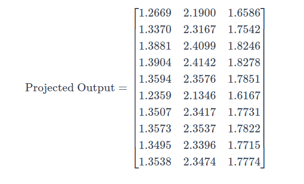
6. Projecting the Attention Output

The attention output is projected back into the embedding space using a projection weight matrix($W_{edO}$).

$$\text{Projected Output} = \text{Attention Output} \cdot W_{edO}$$

Example Projection Matrix $W_{edO}$ :

$$W_{edO} = \begin{bmatrix} 0.3745 & 0.9507 & 0.7320 \ 0.5987 & 0.1560 & 0.1560 \ 0.0581 & 0.8662 & 0.6011 \end{bmatrix}$$
The projected output obtained by projecting back the attention output to the original embedding dimension D is as follows :

$$\text{Projected Output} = \begin{bmatrix} 1.2669 & 2.1900 & 1.6586 \ 1.3370 & 2.3167 & 1.7542 \ 1.3881 & 2.4099 & 1.8246 \ 1.3904 & 2.4142 & 1.8278 \ 1.3594 & 2.3576 & 1.7851 \ 1.2359 & 2.1346 & 1.6167 \ 1.3507 & 2.3417 & 1.7731 \ 1.3573 & 2.3537 & 1.7822 \ 1.3495 & 2.3396 & 1.7715 \ 1.3538 & 2.3474 & 1.7774 \end{bmatrix}$$

7. Feed Forward Network (FFN)

The projected output passes through an FFN:

$$FFN_{output} = (ReLU(\text{Final Attention Output}\times W_{d1}+b_{d1})\times W_{d2} +b_{d2})$$

where $W_{d1}$ and $W_{d2}$ are again weight matrices and $b_{d1}$ and $b_{d2}$ are the biases.

Why is the Feed-Forward Network (FFN) Applied?

The Feed-Forward Network (FFN) acts as a final refinement layer that enhances the decoder’s representations before making predictions. It ensures that each token is processed individually while preserving the broader context learned from attention mechanisms.

1. Fine-Tuning Grammar & Meaning

The FFN helps polish sentence structure by refining syntax (word order) and semantics (meaning).
In machine translation, this ensures fluent and grammatically correct output.

2. Improving Token-Specific Details

Unlike attention, which focuses on relationships between tokens, the FFN processes each token independently.
This allows for word-level adjustments, making sure each token is represented accurately.

3. Capturing Complex Patterns

The FFN introduces nonlinear transformations, enabling it to learn intricate relationships like:
- Tense, gender, and plurality adjustments in translations.
- Handling idioms and nuanced expressions that require deep contextual understanding.

📌 Think of the FFN as a final polish—refining each token’s representation to ensure clarity, coherence, and natural flow before making a prediction.

FeedForward Network Output

The output of the FFN after both transformations is:

$$\text{FFN Output} = \begin{bmatrix} 9.4743 & 8.7558 & 5.8188 \\ 9.9507 & 9.1566 & 6.1009 \\ 10.3006 & 9.4511 & 6.3083 \\ 10.3164 & 9.4643 & 6.3176 \\ 10.1041 & 9.2857 & 6.1918 \\ 9.2654 & 8.5799 & 5.6952 \\ 10.0444 & 9.2355 & 6.1564 \\ 10.0896 & 9.2735 & 6.1832 \\ 10.0366 & 9.2289 & 6.1518 \\ 10.0658 & 9.2535 & 6.1691 \end{bmatrix}$$

8.Residual Connection Output: Preserving and Enriching Context

The residual connection enhances the decoder’s output by adding the projected encoder-decoder attention output back to the FFN output.

Why is this Important?

Preserving Context from Both Sequences
- The decoder generates the output step by step, and it must retain:
  - Token-to-token relationships within the target sequence (from masked attention).
  - Context alignment between the source and target sequences.
- The residual connection ensures that both local (target) and global (source) contexts are maintained.
Enriching Contextual Representations
- Encoder-decoder attention focuses on aligning source and target tokens.
- The residual connection merges this alignment with the decoder’s evolving context, refining the representation for better coherence.
Preparing for Further Processing
- The combined output is passed to the FFN, where:
  - It undergoes grammatical and semantic refinement.
  - Each token’s representation is further enhanced for the next processing stage.

📌 In short, the residual connection prevents information loss, strengthens alignment, and ensures the decoder’s output remains rich in context and meaning.

How is the residual connection computed ?

The residual output obtained is as follows :

$$\text{Residual Output} = \text{Projected Encoder-Decoder Attention Output} + \text{FFN Output}$$

The residual output obtained is as follows :

$$\text{Residual Output} = \begin{bmatrix} 10.7412 & 10.9458 & 7.4774 \\ 11.2877 & 11.4733 & 7.8551 \\ 11.6887 & 11.8611 & 8.1329 \\ 11.7068 & 11.8785 & 8.1454 \\ 11.4635 & 11.6433 & 7.9769 \\ 10.5013 & 10.7145 & 7.3119 \\ 11.3951 & 11.5772 & 7.9295 \\ 11.4469 & 11.6272 & 7.9654 \\ 11.3861 & 11.5685 & 7.9233 \\ 11.4196 & 11.6009 & 7.9465 \end{bmatrix}$$

9. Layer-Normalized Output

The final step involves normalizing the residual output. Layer normalization ensures that the values in a layer's output have a consistent scale and distribution, which is critical for stable and efficient training in neural networks, including transformers.

Why Is Layer Normalization Important ?

Consistent Scale:
- By normalizing the outputs, layer normalization ensures that the scale of values remains consistent across tokens and dimensions, preventing instability caused by large or small activations.
Stable Training:
- Normalized outputs reduce the likelihood of exploding or vanishing gradients during backpropagation, making training more stable.
Effective Gradient Flow:
- Consistent scaling across layers ensures smoother and more predictable gradient updates, improving the model's ability to converge.
Token Independence:
- In transformers, layer normalization is applied independently for each token. This allows the model to normalize the representation of each token without being affected by other tokens in the sequence.

The resulting matrix obtained, after applying layer normalization to the residual output is:

$$\text{Layer Normalized Output} = \begin{bmatrix} 0.6417 & 0.7705 & -1.4123 \\ 0.6506 & 0.7622 & -1.4127 \\ 0.6564 & 0.7567 & -1.4130 \\ 0.6566 & 0.7564 & -1.4130 \\ 0.6532 & 0.7597 & -1.4129 \\ 0.6375 & 0.7745 & -1.4120 \\ 0.6522 & 0.7607 & -1.4128 \\ 0.6529 & 0.7599 & -1.4129 \\ 0.6520 & 0.7608 & -1.4128 \\ 0.6525 & 0.7603 & -1.4128 \end{bmatrix}$$

Layer normalization marks the end of forward propagation in the decoder, leading to the final step—projecting the normalized output onto the target vocabulary space to predict the next token.

Final Projection to the Vocabulary Space

The final step in the decoder is to project the layer-normalized output into the target vocabulary space to generate predictions for the next token.

How Does This Projection Work?

Decoder Output Transformation
- The decoder produces an output matrix of size $M \times D$, where:
  - $M$ is the number of tokens in the generated sequence.
  - $D$ is the embedding dimension.
Mapping to Vocabulary Space
- A learnable weight matrix $W_{\text{vocab}} $ (of size $D \times V_c$, where $V_c$ is the vocabulary size) transforms the decoder's output into a probability distribution over all possible tokens.
- Each token representation is projected from dimension $D$ → dimension $V_c$, resulting in a matrix of size $M \times V_c$.

Purpose of the Projection

Aligns the decoder’s contextualized output with the target vocabulary.
Produces a probability distribution over the vocabulary for each token in the sequence.
Ensures the model can sample or select the most likely next token during generation.

Computing Logits & Softmax

The projected output, referred to as logits, is computed as:

$$\text{logits} = \text{Layer Normalized Output} \times W_{\text{vocab}} + b_{\text{vocab}}$$

These logits are then passed through a softmax function to obtain probabilities for each token:

$$P(y_t \mid y_{

Each row in the resulting matrix represents the probability distribution over the vocabulary for a given token position in the output sequence.
This is nothing but the probability of each token(column) in the target vocabulary being the correct token for that position in the target sequence.
The highest probability token is selected as the predicted output.

Why Softmax?

Converts raw logits into interpretable probability scores.
Ensures that the sum of probabilities across the vocabulary is 1 for each token position.
Helps in selecting the most likely next token during training and inference.

Conclusion & Next Steps

With the forward propagation in the Transformer decoder complete, we now have a detailed understanding of how the model processes information at each step. The decoder retrieves relevant context from the encoder, applies attention mechanisms, and refines token representations before making predictions.

However, the Transformer is only as good as its training process. To improve accuracy and minimize prediction errors, we must update the model’s parameters using backpropagation. In the next and final part of this series, we will delve into the backpropagation process and inference phase, exploring how gradients are computed, weights are adjusted, and how the model ultimately learns to generate high-quality outputs.

Stay tuned for the next blog, where we unravel the final part of the crucial training phase of Transformers! 🚀

Transformer Decoder: Forward Pass Mechanism and Key Insights (part 6)

Table of contents