Introduction

Support Vector Machines (SVM) are one of the most powerful and versatile supervised learning algorithms used for classification and regression tasks. They are known for their effectiveness in high-dimensional spaces and work well even when the number of dimensions is greater than the number of samples.

SVM Terminology:

• Hyperplane: A decision boundary separating different classes in feature space, represented by the equation wx + b = 0 in linear classification.

• Support Vectors: The closest data points to the hyperplane, crucial for determining the hyperplane and margin in SVM.

• Margin: The distance between the hyperplane and the support vectors. SVM aims to maximize this margin for better classification performance.

• Kernel: A function that maps data to a higher-dimensional space, enabling SVM to handle non-linearly separable data.

• Hard Margin: A maximum-margin hyperplane that perfectly separates the data without misclassifications.

• Soft Margin: Allows some misclassifications by introducing slack variables, balancing margin maximization and misclassification penalties when data is not perfectly separable.

• C: A regularization term balancing margin maximization and misclassification penalties. A higher C value enforces a stricter penalty for misclassifications.

• Hinge Loss: A loss function penalizing misclassified points or margin violations, combined with regularization in SVM.

• Dual Problem: Involves solving for Lagrange multipliers associated with support vectors, facilitating the kernel trick and efficient computation.

---

1. What is Support Vector Machine (SVM)?

SVM is a supervised learning algorithm that aims to find the optimal hyperplane that separates data points into different classes. It maximizes the margin between the classes, ensuring that the closest data points (support vectors) are as far away as possible from the decision boundary.

1.1 Why Use SVM?

• High Accuracy: Effective in high-dimensional spaces and performs well with a clear margin of separation.

• Robustness: Works well with both linearly and non-linearly separable data using the kernel trick.

• Versatility: Can be used for classification, regression, and outlier detection.

---

2. How Does SVM Work?

SVM tries to find the optimal hyperplane that best separates the data into different classes.

2.1 Hyperplane and Decision Boundary:

A hyperplane is a decision boundary that separates data points of different classes. In 2D, it's a line; in 3D, it's a plane; and in N-dimensional space, it's an N-1 dimensional hyperplane.
The key idea behind the SVM algorithm is to find the hyperplane that best separates two classes by maximizing the margin between them. This margin is the distance from the hyperplane to the nearest data points (support vectors) on each side.

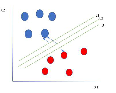
The best hyperplane, also known as the “hard margin,” is the one that maximizes the distance between the hyperplane and the nearest data points from both classes. This ensures a clear separation between the classes. So, from the above figure, we choose L2 as hard margin.

2.2 Support Vectors:

Support vectors are the data points that lie closest to the hyperplane. These points influence the position and orientation of the hyperplane.

2.3 Maximum Margin Classifier:

The goal of SVM is to find the hyperplane with the maximum margin, which is the maximum distance between the support vectors of the two classes. This maximizes the classifier's robustness and generalization.
A soft margin allows for some misclassifications or violations of the margin to improve generalization. The SVM optimizes the following equation to balance margin maximization and penalty minimization:

The penalty used for violations is often hinge loss, which has the following behavior:

• If a data point is correctly classified and within the margin, there is no penalty (loss = 0).

• If a point is incorrectly classified or violates the margin, the hinge loss increases proportionally to the distance of the violation.

---

3. Mathematical Intuition Behind SVM

Consider a binary classification problem with two classes, labeled as +1 and -1. We have a training dataset consisting of input feature vectors X and their corresponding class labels Y.

The equation for the linear hyperplane can be written as:

Where:

• w is the normal vector to the hyperplane (the direction perpendicular to it).

• b is the offset or bias term, representing the distance of the hyperplane from the origin along the normal vector w.

3.1 Distance from a Data Point to the Hyperplane

The distance between a data point x_i and the decision boundary can be calculated as:

where ||w|| represents the Euclidean norm of the weight vector w. Euclidean norm of the normal vector W

3.2 Linear SVM Classifier

Distance from a Data Point to the Hyperplane:

Where y^y^​ is the predicted label of a data point.

3.3 Optimization Problem for SVM

For a linearly separable dataset, the goal is to find the hyperplane that maximizes the margin between the two classes while ensuring that all data points are correctly classified. This leads to the following optimization problem:

Subject to the constraint:

Where:

• yi​​ is the class label (+1 or -1) for each training instance.

• xi is the feature vector for the i-th training instance.

• mm is the total number of training instances.

The condition yi(wTxi+b)≥1 ensures that each data point is correctly classified and lies outside the margin.

3.4 Decision Boundary:

Once the dual problem is solved, the decision boundary is given by:

Where w is the weight vector, xx is the test data point, and b is the bias term.

Finally, the bias term b is determined by the support vectors, which satisfy:

Where xi is any support vector.

This completes the mathematical framework of the Support Vector Machine algorithm, which allows for both linear and non-linear classification using the dual problem and kernel trick.

3.5 Classification Rule:

• If f(x)>0f(x) > 0, classify as Class 1

• If f(x)<0f(x) < 0, classify as Class 2

3.6 Soft Margin and C Parameter:

In the presence of outliers or non-separable data, the SVM allows some misclassification by introducing slack variables ζiζi​​. The optimization problem is modified as:

Subject to the constraints:

Where:

• C is a regularization parameter that controls the trade-off between margin maximization and penalty for misclassifications.

• ζi are slack variables that represent the degree of violation of the margin by each data point.

To handle noisy data and misclassifications, SVM uses a Soft Margin approach with a regularization parameter C:

• C controls the trade-off between maximizing the margin and minimizing the classification error.

• High C: Less margin, fewer misclassifications (overfitting risk).

• Low C: Larger margin, more misclassifications (better generalization).

Dual Problem for SVM

The dual problem involves maximizing the Lagrange multipliers associated with the support vectors. This transformation allows solving the SVM optimization using kernel functions for non-linear classification.

The dual objective function is given by:

Where:

• αi​​ are the Lagrange multipliers associated with the i-th training sample.

• ti is the class label for the i-th training sample (+1 or −1).

• K(xi,xj) is the kernel function that computes the similarity between data points xi​​ and xj. The kernel allows SVM to handle non-linear classification problems by mapping data into a higher-dimensional space.

The dual formulation optimizes the Lagrange multipliers αiαi​​, and the support vectors are those training samples where αi>0αi​>0.

---

4. Kernels in SVM

4.1 Why Use Kernels?

SVM can efficiently handle non-linearly separable data using the Kernel Trick, which transforms the input space into a higher-dimensional feature space where a linear separator is possible.

4.2 Common Kernel Functions:

1. Linear Kernel: Used when data is linearly separable.

2. Polynomial Kernel: Useful for complex boundaries.

• d = Degree of the polynomial

• c = Constant term (controls flexibility)

3. Radial Basis Function (RBF) Kernel: For non-linear decision boundaries.

• γ controls the influence of a single training example.

4. Sigmoid Kernel: Similar to a neural network activation function.

---

5. Hyperparameters and Tuning

5.1 Key Hyperparameters:

• C (Regularization Parameter): Controls the trade-off between maximizing the margin and minimizing misclassification.

• Kernel: Choice of kernel function (linear, polynomial, RBF, sigmoid).

• Gamma (RBF Kernel): Controls the influence of a single training example.

• Degree (Polynomial Kernel): Degree of the polynomial kernel function.

5.2 Hyperparameter Tuning:

• Use Grid Search or Random Search with Cross-validation to find the best combination of hyperparameters.

---

6. Advantages and Disadvantages

6.1 Advantages:

• Effective in High Dimensions: Works well with high-dimensional data.

• Robust to Overfitting: Especially with a proper choice of C and kernel.

• Memory Efficient: Uses support vectors for decision making.

6.2 Disadvantages:

• Computationally Expensive: Especially for large datasets.

• Difficult to Interpret: Decision boundary is not easily interpretable.

• Requires Feature Scaling: Input features need to be normalized.

---

7. Types pf Support Vector Machine

Based on the nature of the decision boundary, Support Vector Machines (SVM) can be divided into two main parts:

Linear SVM:

Linear SVMs use a linear decision boundary to separate the data points of different classes. When the data can be precisely linearly separated, linear SVMs are very suitable. This means that a single straight line (in 2D) or a hyperplane (in higher dimensions) can entirely divide the data points into their respective classes. A hyperplane that maximizes the margin between the classes is the decision boundary.

Non-Linear SVM:

Non-Linear SVM can be used to classify data when it cannot be separated into two classes by a straight line (in the case of 2D). By using kernel functions, nonlinear SVMs can handle non-linearly separable data. The original input data is transformed by these kernel functions into a higher-dimensional feature space, where the data points can be linearly separated. A linear SVM is used to locate a nonlinear decision boundary in this modified space.

---

8. Implementation in Python

Let's implement an SVM Classifier using Scikit-learn:

# Import necessary libraries
import numpy as np
import matplotlib.pyplot as plt
from sklearn import datasets
from sklearn.model_selection import train_test_split
from sklearn.svm import SVC
from sklearn.metrics import accuracy_score, classification_report, confusion_matrix
import seaborn as sns

# Load Dataset
iris = datasets.load_iris()
X = iris.data[:, :2]  # Only using first two features for visualization
y = iris.target

# Split data into training and testing sets
X_train, X_test, y_train, y_test = train_test_split(X, y, test_size=0.3, random_state=42)

# Create SVM Classifier with RBF kernel
model = SVC(kernel='rbf', gamma='auto', C=1.0)
model.fit(X_train, y_train)

# Make predictions
y_pred = model.predict(X_test)

# Evaluate Model
print("Accuracy:", accuracy_score(y_test, y_pred))
print("Classification Report:\n", classification_report(y_test, y_pred))
print("Confusion Matrix:\n", confusion_matrix(y_test, y_pred))

# Visualize Decision Boundary
plt.scatter(X_test[:, 0], X_test[:, 1], c=y_pred, cmap='coolwarm')
plt.title('SVM Decision Boundary')
plt.show()

---

9. Real-world Applications

• Image Classification: Object detection and facial recognition.

• Text Categorization: Spam detection and sentiment analysis.

• Bioinformatics: Protein classification and gene expression analysis.

• Finance: Credit risk analysis and stock market prediction.

• Healthcare: Disease diagnosis and medical image analysis.

---

10. Tips for Better Performance

• Feature Scaling: SVM is sensitive to feature scaling, so normalize the input features.

• Kernel Selection: Experiment with different kernels (RBF, Polynomial) to find the best fit.

• Hyperparameter Tuning: Use Grid Search or Random Search for optimal C and gamma values.

• Cross-validation: Use k-fold cross-validation to avoid overfitting.

---

11. Conclusion

Support Vector Machines are powerful classifiers known for their robustness, high accuracy, and ability to handle high-dimensional data. Using the right kernel and hyperparameters can significantly improve performance.