Principal Component Analysis (PCA) – Unleashing the Power of Dimensionality Reduction
 Tushar Pant
Table of contents
- Why Use PCA?
- 1. What is Principal Component Analysis (PCA)?
- 2. How PCA Works
- 3. Mathematical Concepts Behind PCA
- 4. Choosing the Number of Principal Components
- 5. Advantages and Disadvantages
- 6. PCA vs Other Dimensionality Reduction Techniques
- 7. Implementation of PCA in Python
- 8. Real-World Applications
- 9. Conclusion

Introduction
In the era of big data, high-dimensional datasets are common. However, working with too many features can be challenging due to the Curse of Dimensionality, increased computational cost, and risk of overfitting. Principal Component Analysis (PCA) is a powerful dimensionality reduction technique that transforms high-dimensional data into a lower-dimensional space while retaining as much variability as possible.
Why Use PCA?
Dimensionality Reduction: Reduces the number of features while preserving important information.
Noise Reduction: Filters out noise and redundant features.
Visualization: Enables visualization of high-dimensional data in 2D or 3D.
Faster Computation: Speeds up training for machine learning models.
1. What is Principal Component Analysis (PCA)?
Principal Component Analysis (PCA) is an unsupervised linear transformation technique that projects data onto a new coordinate system, maximizing variance along the principal components (axes).
1.1 Key Characteristics of PCA:
Orthogonal Transformation: Transforms correlated features into linearly uncorrelated components.
Principal Components: New axes (linear combinations of original features) that capture maximum variance.
Ranked by Importance: Components are ordered by the amount of variance they capture.
Feature Reduction: Retains only the most important components, reducing dimensionality.
1.2 When to Use PCA?
When you have high-dimensional data (e.g., images, gene expression).
When features are highly correlated.
When you want to visualize complex data in 2D or 3D.
When you need to speed up machine learning models by reducing input features.
2. How PCA Works
PCA involves the following steps:
Step 1: Standardize the Data
PCA makes sure all features (e.g., height, weight, age) are on the same scale. Since PCA is sensitive to the scale of features, standardize the data to have a mean of 0 and a standard deviation of 1:

Where:
X = Original data.
μ = Mean of each feature.
σ = Standard deviation of each feature.
Step 2: Calculate the Covariance Matrix
Compute the Covariance Matrix to understand the relationships between features:

Where:
C = Covariance matrix.
N = Number of data points.
The value of covariance can be positive, negative, or zeros.
Positive: As the x1 increases x2 also increases.
Negative: As the x1 increases x2 also decreases.
Zeros: No direct relation.
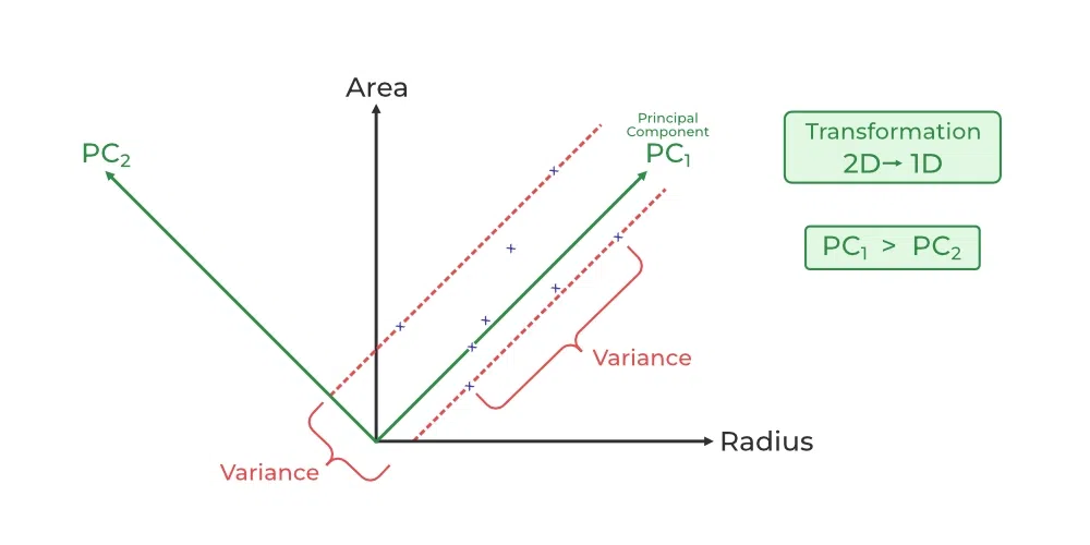
Step 3: Find the “magic Directions”
PCA identifies new axes (like rotating a camera) where the data spreads out the most:
1st Principal Component (PC1): The direction of maximum variance (most spread).
2nd Principal Component (PC2): The next best direction, perpendicular to PC1, and so on.
These directions are calculated using Eigenvalues and Eigenvectors where: eigenvectors (math tools that find these axes), and their importance is ranked by eigenvalues (how much variance each captures).
For a square matrix A, an eigenvector X (a non-zero vector) and its corresponding eigenvalue λ (a scalar) satisfy:

Where:
C = Covariance matrix.
v = Eigenvector.
λ = Eigenvalue.
This means:
When C acts on v, it only stretches or shrinks v by the scalar λ.
The direction of v remains unchanged (hence, eigenvectors define “stable directions” of C).
Step 4: Sort Eigenvalues and Eigenvectors
Sort the eigenvalues in descending order to rank the principal components by importance.
Rearrange the corresponding eigenvectors accordingly.
Step 5: Select Principal Components
Choose the top k eigenvectors corresponding to the largest eigenvalues.
This forms the Projection Matrix:

Step 6: Project the Data
Transform the original data into the new space:

Where:
Z = Transformed data in the reduced space.
W = Projection matrix.
3. Mathematical Concepts Behind PCA
3.1 Variance Maximization
PCA seeks to maximize the variance of the projected data to retain the most significant patterns.
3.2 Orthogonal Components
All principal components are orthogonal (uncorrelated) to each other.
3.3 Explained Variance
Represents the proportion of total variance captured by each component.
Used to determine the number of components to retain.

4. Choosing the Number of Principal Components
Use the Explained Variance Ratio to choose components capturing sufficient variance.
Cumulative Explained Variance is plotted to decide the optimal number of components (e.g., 95% variance).
Use the Scree Plot to observe the "elbow point" where adding more components has diminishing returns.
5. Advantages and Disadvantages
5.1 Advantages:
Dimensionality Reduction: Reduces features while retaining most information.
Noise Reduction: Eliminates noisy and redundant features.
Improved Performance: Enhances speed and efficiency of machine learning models.
Visualization: Helps in visualizing high-dimensional data.
5.2 Disadvantages:
Loss of Interpretability: Transformed components are linear combinations of original features.
Linear Assumption: Assumes linear relationships between features.
Sensitive to Scaling: Requires standardized data for meaningful results.
6. PCA vs Other Dimensionality Reduction Techniques
| Feature | PCA | t-SNE | LDA |
| Type | Linear | Non-linear | Supervised |
| Preserves Variance | Yes | No | No |
| Interpretability | Low | Very Low | Moderate |
| Scalability | High | Low | Moderate |
7. Implementation of PCA in Python
# Import Libraries
import numpy as np
import matplotlib.pyplot as plt
from sklearn.decomposition import PCA
from sklearn.datasets import load_iris
# Load Dataset
data = load_iris()
X = data.data
y = data.target
# Standardize the Data
from sklearn.preprocessing import StandardScaler
X_std = StandardScaler().fit_transform(X)
# Standardize the Data
from sklearn.preprocessing import StandardScaler
X_std = StandardScaler().fit_transform(X)
# Apply PCA
pca = PCA(n_components=2)
X_pca = pca.fit_transform(X_std)
# Plot the Results
plt.figure(figsize=(8,6))
plt.scatter(X_pca[:, 0], X_pca[:, 1], c=y, cmap='viridis', edgecolor='k', s=100)
plt.title('PCA - Iris Dataset')
plt.xlabel('Principal Component 1')
plt.ylabel('Principal Component 2')
plt.grid(True)
plt.show()

8. Real-World Applications
Image Compression: Reducing image dimensions while preserving quality.
Face Recognition: Reducing complexity for faster recognition.
Finance: Portfolio analysis and risk management.
Genomics: Analyzing high-dimensional gene expression data.
9. Conclusion
Principal Component Analysis (PCA) is a powerful and widely-used dimensionality reduction technique that transforms high-dimensional data into a lower-dimensional space while retaining maximum variance.
Subscribe to my newsletter
Read articles from Tushar Pant directly inside your inbox. Subscribe to the newsletter, and don't miss out.
Written by
Tushar Pant
Tushar Pant
Cloud and DevOps Engineer with hands-on expertise in AWS, CI/CD pipelines, Docker, Kubernetes, and Monitoring tools. Adept at building and automating scalable, fault-tolerant cloud infrastructures, and consistently improving system performance, security, and reliability in dynamic environments.