Objective

Poor road conditions in surface mining can significantly impact safety, equipment longevity, and overall operational efficiency. Some common issues include:

Improper grading: Leads to water pooling, potholes, and erosion.
Soft spots and ruts: Cause uneven loading on tires and suspension systems, leading to premature wear and tear.
Frequent repairs needed: Increases downtime and operational costs.
Inefficient haul cycles: Poor roads slow down production and reduce fuel efficiency.
Steep inclines and sharp turns: Increase the risk of rollovers and equipment accidents.

Therefore, maintaining an acceptable level of efficiency for the entire road network by adopting effective road pavement monitoring and maintenance programs becomes a major challenge.

The objective of this work is to develop a low-cost and reliable system able to carry out real-time screening of road pavement conditions. The data are acquired with accelerometers mounted on a vehicle, and the data are analyzed by machine learning.

Accelerometers Signal

Accelerometer data is useful for road pavement monitoring because it captures vibrations, shocks, and surface irregularities that indicate road conditions. Here’s why it helps:

1. Detecting Surface Irregularities

When a vehicle drives over potholes, cracks, ruts, or bumps, the accelerometer detects sudden vertical and horizontal accelerations.
Larger vibrations indicate severe damage, while smaller variations may suggest surface roughness or early wear.

2. Cost-Effective & Scalable

Traditional pavement assessments rely on LIDAR, laser profilometers, or high-resolution cameras, which are expensive.
Accelerometers are low-cost sensors that can be easily deployed on multiple vehicles for large-scale monitoring.

Short-Time Fourier Transform (STFT)

A Short-Time Fourier Transform (STFT) of the accelerometer signal works well for road condition monitoring because it provides a time-frequency representation of the signal, helping to analyze how different vibration frequencies change over time. Here's why STFT is useful.

Road Defects Have Distinct Frequency Signatures

STFT Solves This Problem by Adding Frequency Information

Instead of just plotting acceleration vs. time, STFT transforms the signal into a time-frequency spectrogram.
This helps distinguish between:
- Sharp, short bursts of high-frequency energy → Likely a pothole.
- Longer-lasting, periodic vibrations → Likely corrugations or rough roads.
- Low-frequency oscillations → Normal vehicle motion.
- More random, broadband frequency content. —> Loose gravel

Capturing Localized Events (Time-Frequency Analysis)

A standard Fourier Transform (FT) gives only a global frequency spectrum, losing time-related information.
STFT applies a moving window to analyze the signal in small time segments, preserving time information.
This allows detection of transient events like sudden jolts from potholes, which might otherwise be lost in a full FT.

For example, a sharp pothole impact will appear as a short burst of high-frequency energy, while a washboard road will show repeating frequency patterns over time.

Differentiating Road Anomalies from Vehicle Motion

Mining trucks have inherent vibrations due to engine and suspension movement.
These background vibrations occur at consistent, lower frequencies.
STFT helps filter out these steady-state vibrations and isolate high-frequency spikes or irregular patterns caused by actual road issues.

Feature Extraction for Machine Learning

The STFT spectrogram can be used as input for ML models to classify road conditions.
Features like spectral entropy, peak frequency, and energy distribution help distinguish between smooth and rough roads.

How STFT Provides a Time-Frequency Representation

STFT divides the signal into short time segments and applies a Fourier Transform to each.
This results in a spectrogram, which is a 2D representation where:
- X-axis = Time
- Y-axis = Frequency
- Color/Intensity = Energy at that frequency

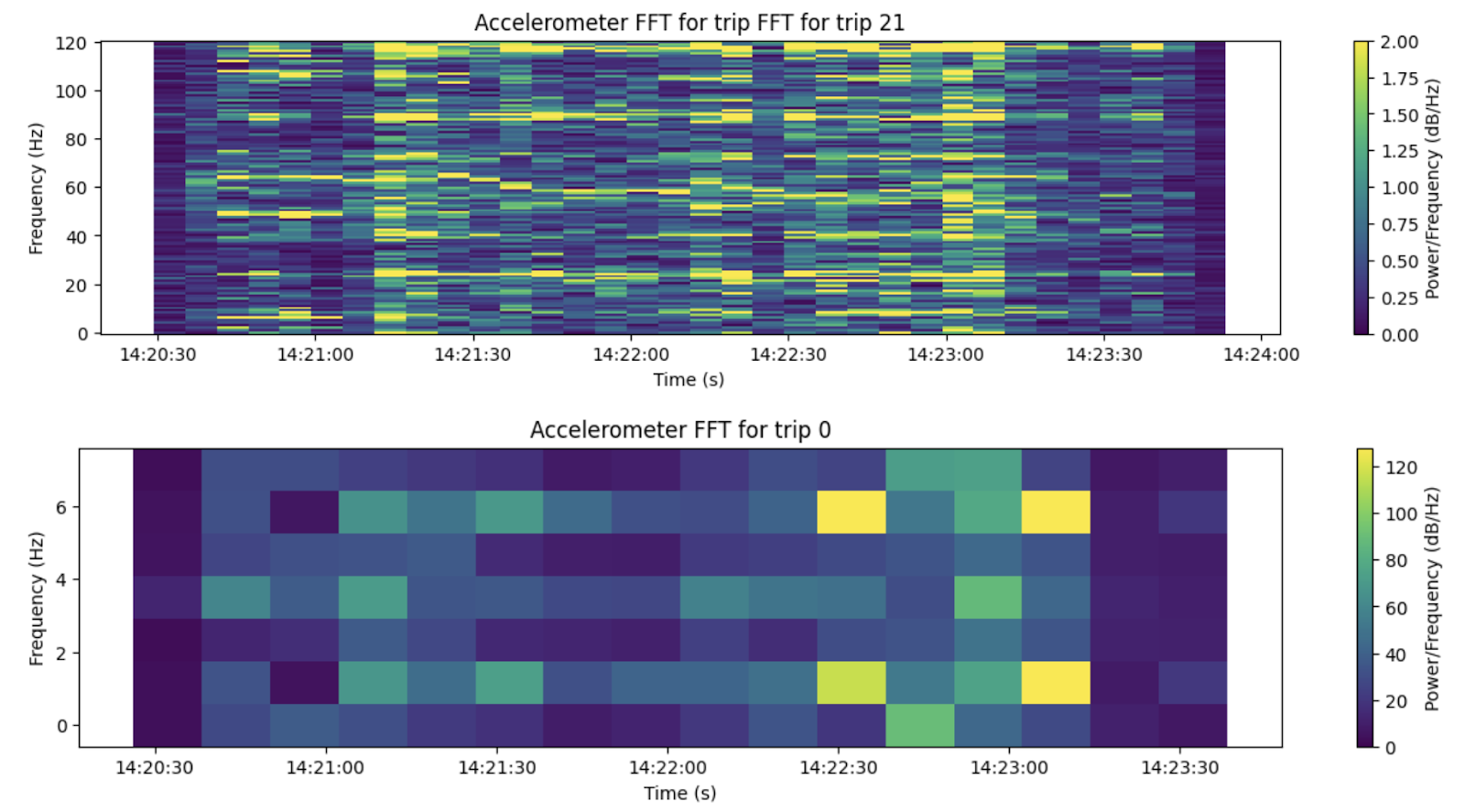
An example visualization!

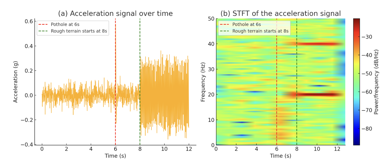
Acceleration signal over time: The first plot shows a relatively smooth signal initially. At 6 seconds, there is a sharp spike due to a pothole impact, followed by a transition to rough terrain at 8 seconds, where the signal becomes more erratic and higher in frequency.
STFT (Short-Time Fourier Transform) Spectrogram: The second plot highlights the frequency content over time. Initially, low frequencies dominate. At 6 seconds, there's a brief high-energy event (pothole) across a broad range of frequencies. After 8 seconds, higher frequency components become more pronounced, indicating rough terrain.

Feature Engineering

Spectral Entropy

Spectral entropy is a measure of the disorder or randomness in the frequency domain of a signal.

Intuition

If the signal contains a single frequency component, its spectral entropy will be low because most of the power is concentrated at one frequency.
If the signal has a broad spectrum with many frequency components, the spectral entropy will be high, indicating a more random or complex structure.

How Spectral Entropy Captures Changes in Road conditions?

Spectral entropy measures the distribution of energy across the frequency spectrum:

For a smooth road: The acceleration signal is mostly low-frequency, with low spectral entropy because power is concentrated in a few frequency bins.
For a pothole: A sudden impact creates a sharp peak in the frequency domain, temporarily increasing spectral entropy.
For rough terrain: The signal contains a wider range of frequencies, leading to higher spectral entropy over a longer duration.

Mathematical Definition

Frame: The total time window that represents the smallest unit for feature computation.

Segment: A division of the frame along the time axis (x-axis). The STFT applies the discrete Fourier transform (DFT) to the signal within each segment.

Block: A further subdivision along the frequency axis (y-axis), grouping the frequency range into discrete bins within each segment.
Each block in this STFT matrix is defined by (p,u) where 0 ≤ p ≤ P−1 and 0 ≤ u ≤U−1, with P representing the number of segments within the acquired frame and U denoting the number of frequency samples within each segment.

The STFT matrix is divided into submatrices. The energy contained in each submatrix (i, j) is computed as

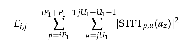
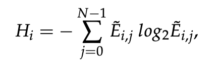
where E ̃i,j is a scaled (normalized) version of Ei,j such that ∑N−1 E ̃i,j \= 1 for 0 ≤ i ≤ M − 1.

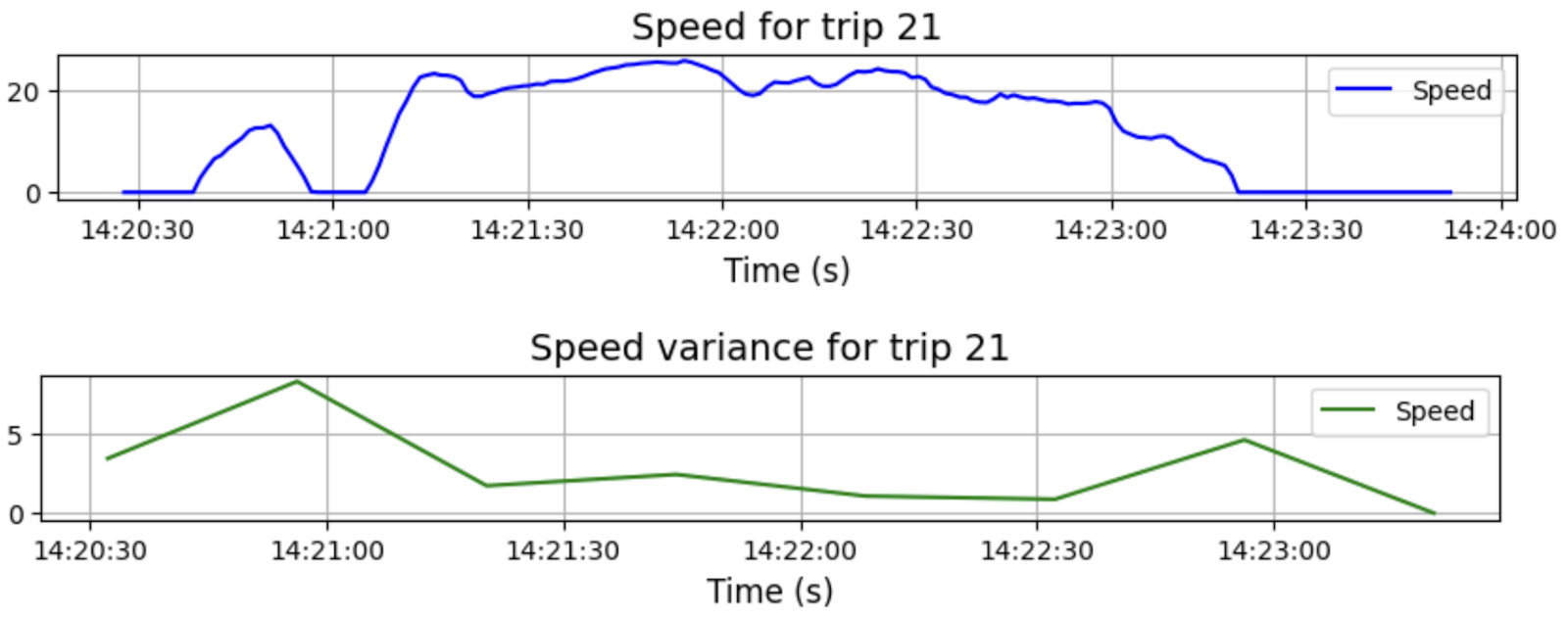
Speed Variation

The speed of a vehicle is also aﬀected by the road condition. Two key observations:

Damaged Roads Reduce Speed – Vehicles tend to slow down when traveling on roads with larger damaged segments.
Potholes Cause Sudden Vibrations – On smoother roads, vehicles traveling at higher speeds experience noticeable vibrations when encountering potholes or small damaged segments.

These insights highlight how speed variation can be a useful parameter for road categorization, helping identify road quality based on vehicle movement patterns.

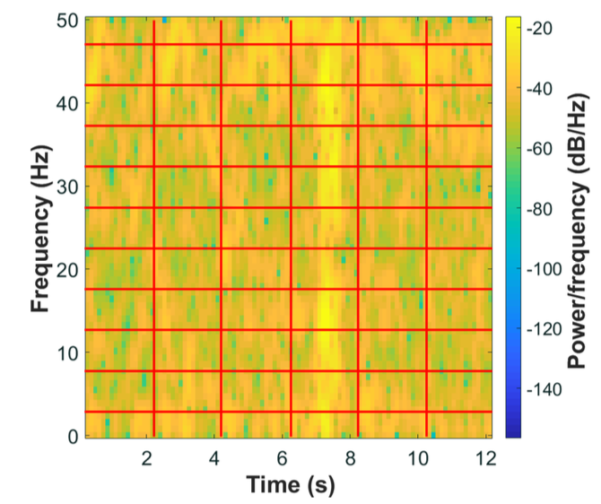
Illustration of the above features for a time frame of a particular trip:

The above diagram shows the block energy aggregated from the SFTP diagram over it.

Other Key Sensors for this System

GPS Sensors to map detected anomalies to specific locations.
- By combining accelerometer readings with GPS coordinates, the system can generate a real-time road quality map.

Model Selection

Since there is no labeled data available to indicate the actual condition of the mining road, an unsupervised approach is necessary.
This involves applying a combination of the Self-Organizing Map (SOM) and k-means clustering algorithms to features extracted from GPS and accelerometer data for road condition monitoring.
The SOM algorithm differentiates between damaged and non-damaged road segments, while the k-means algorithm further classifies the roughness levels of the non-damaged road segments.

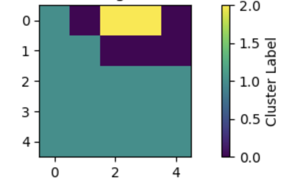
SOM Modelling

We used the network of 5×5 neurons for small mining areas and 10x10 neurons for larger mining areas.
We analyze the codebook, distance, and hit count matrices of SOM networks trained on trip data. Neurons linked to damaged road segments exhibit high distances from their neighbors and have significantly lower hit counts due to the lower proportion of damaged segments in the overall stretch. These segments can be efficiently identified using a distance or hit count threshold.
The codebook matrix (CC) is split into two parts: Cd for damaged road segments and Cd′ for other segments. Similarly, the distance (D) and hit count (H) matrices are divided. No further processing is done for damaged segments (Cd,Dd,Hd), but the non-damaged segments (Cd′,Dd′,Hd′) undergo k-means clustering (in the next section) to classify road roughness levels (smooth, moderate, high).

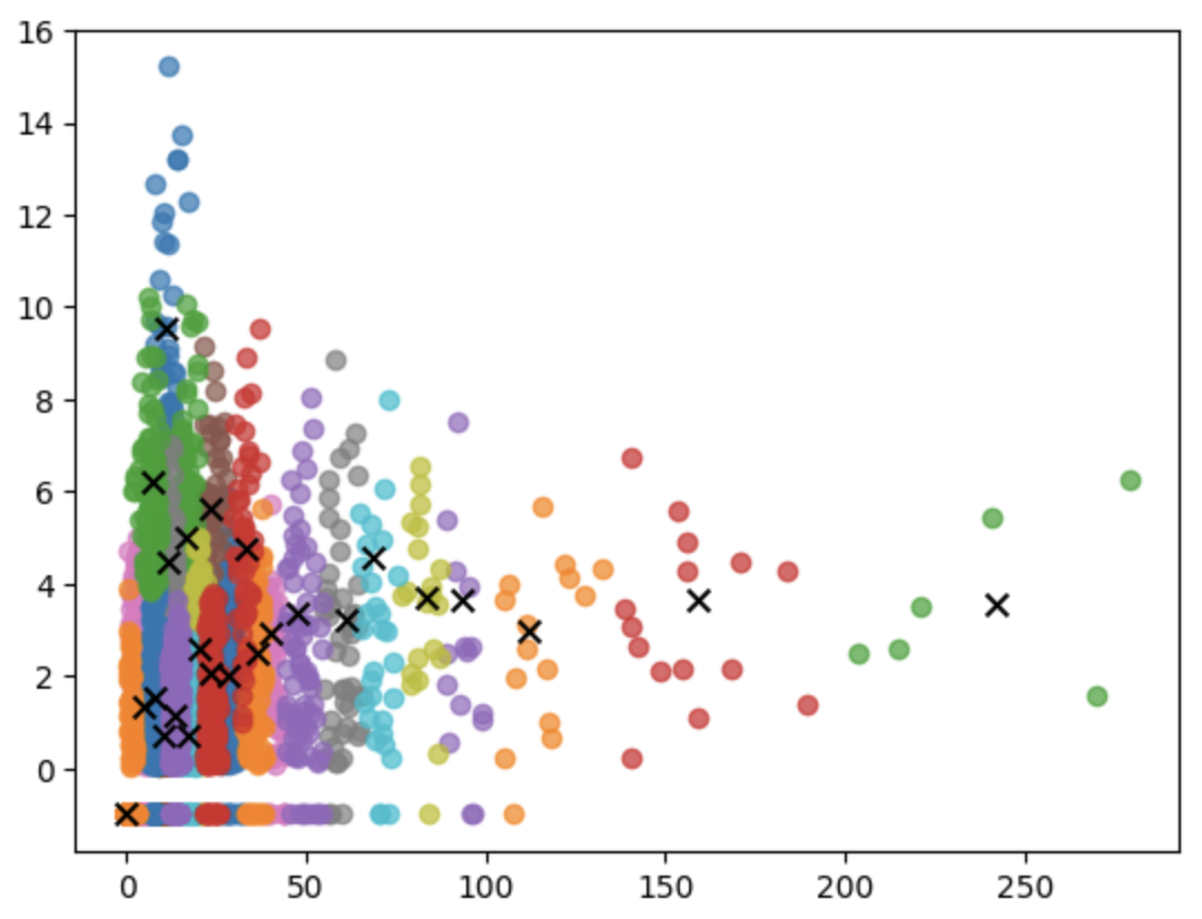
K-Means Clustering

The non-damaged segments from SOM (Cd′,Dd′,Hd′) undergo k-means clustering to classify road roughness levels - smooth (green), moderate (yellow), high (orange). The damaged road segments inferred from SOM are labelled as red.

Geo-Coordinate Tagging & Patches

The next step involves mapping each sample from the Feature Data to its corresponding temporal cluster and also associating it with the vehicle's GPS coordinates during that time window.
To streamline computations, geo-coordinates are converted into geohashes. We then perform a frequency count of each geohash’s occurrence within a cluster and use a color-coding heuristic based on these counts to assign a final color to each geohash.
Finally, DBSCAN is applied to geohashes of the same color to identify continuous sequences of geohashes thereby creating bigger road patches.
Each identified road patch is assigned a unique identifier and stored in our database. This ensures that when the algorithm runs daily, it can first check for existing patches that closely overlap with newly detected ones and reuse them instead of creating duplicates.

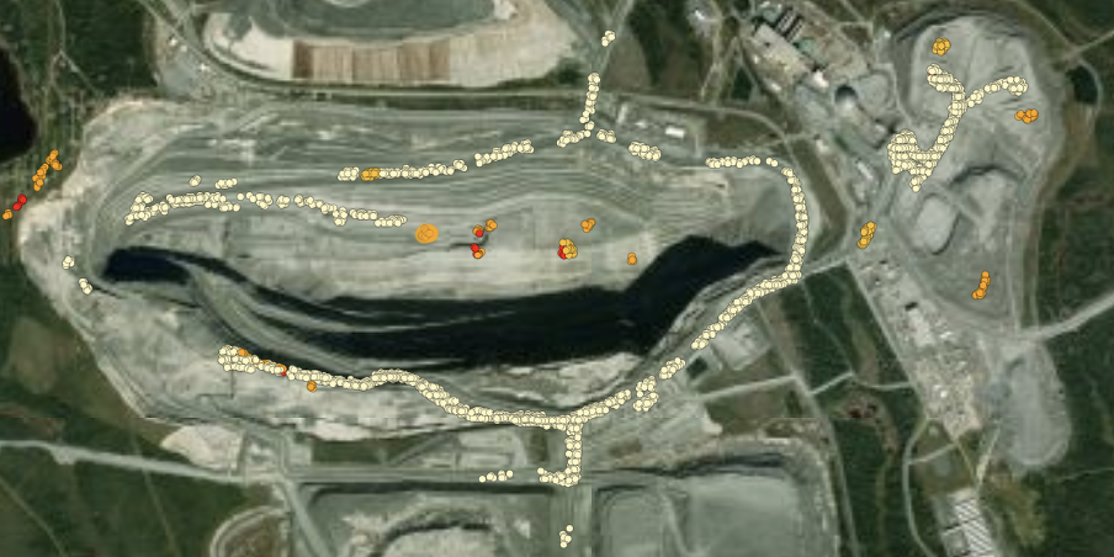
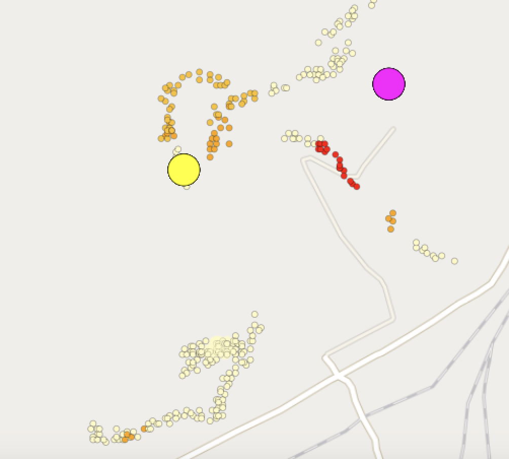
Final Result: Road Quality Heat Map

The images below illustrate examples of how we visualize the patches on maps. To maintain clarity and focus, we exclude smooth patches (green ones) from visualization, as our primary objective is to highlight rough patches.

Future Work

Collect feedback from the mining areas to measure the accuracy of the results.
Explore other techniques to improve the accuracy.

How to Detect Poor Road Conditions in Surface Mining Sites

Table of contents