1. Introduction

In the field of speech processing, converting continuous signals into a form that can be processed by machines is crucial. This digital representation of speech involves three fundamental concepts: waveforms, sampling, and quantization. These concepts serve as the foundation for various speech processing tasks like Automatic Speech Recognition (ASR), speech synthesis, and audio compression. In this blog, we’ll explore each concept in detail and understand their significance.

2. Waveforms

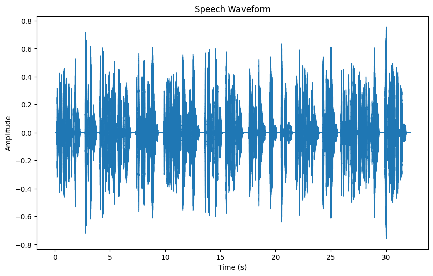
A waveform is a graphical representation of a speech signal in the time domain. It shows how the amplitude of the signal varies over time. When you record a human voice, the result is a waveform — a physical sound wave that we can manipulate digitally.

Waveforms allow us to understand the general shape and intensity of sound at any given moment. Speech waveforms typically exhibit periodic patterns for vowels and irregular shapes for consonants. These characteristics make waveforms essential for tasks like signal analysis and feature extraction.

Visualizing Waveforms:

We can visualize a waveform of a speech signal using Python libraries like librosa and matplotlib. Here's an example:

pythonCopyEditimport librosa
import matplotlib.pyplot as plt

# Load an example speech signal
y, sr = librosa.load("data/example_audio.wav", sr = None)

# Visualize the waveform
plt.figure(figsize=(10, 6))
librosa.display.waveshow(y, sr=sr)
plt.title("Speech Waveform")
plt.xlabel("Time (s)")
plt.ylabel("Amplitude")
plt.show()

In this plot, the x-axis represents time, and the y-axis shows the amplitude. The waveform tells us how the sound changes over time, revealing how speech flows.

3. Sampling

Sampling refers to the process of converting a continuous signal (like a real-world sound wave) into a discrete signal by measuring the amplitude at regular intervals. The rate at which we take these samples is known as the sampling rate or sampling frequency.

To accurately represent a continuous signal, the sampling rate must be sufficient to capture its details. According to the Nyquist theorem, the sampling rate should be at least twice the highest frequency in the signal to avoid aliasing — the distortion that occurs when the signal is under-sampled.

In speech processing, common sampling rates are 8 kHz (for telephony) and 44.1 kHz (for high-quality audio like CDs).

Effect of Sampling Rate:

Let's experiment with the impact of different sampling rates on speech signals. By resampling, we can observe how the signal changes when we reduce or increase the sampling rate.

import librosa
import matplotlib.pyplot as plt

y,sr = librosa.load("data/example_audio.wav", sr=None)

# Resample the signal to 8 kHz
y_resampled_8k = librosa.resample(y, orig_sr = sr, target_sr = 8000)

# Plot the resampled signal
plt.figure(figsize=(10, 6))
librosa.display.waveshow(y_resampled_8k, sr=8000)
plt.title("Resampled Speech Signal at 8 kHz")
plt.xlabel("Time (s)")
plt.ylabel("Amplitude")
plt.show()

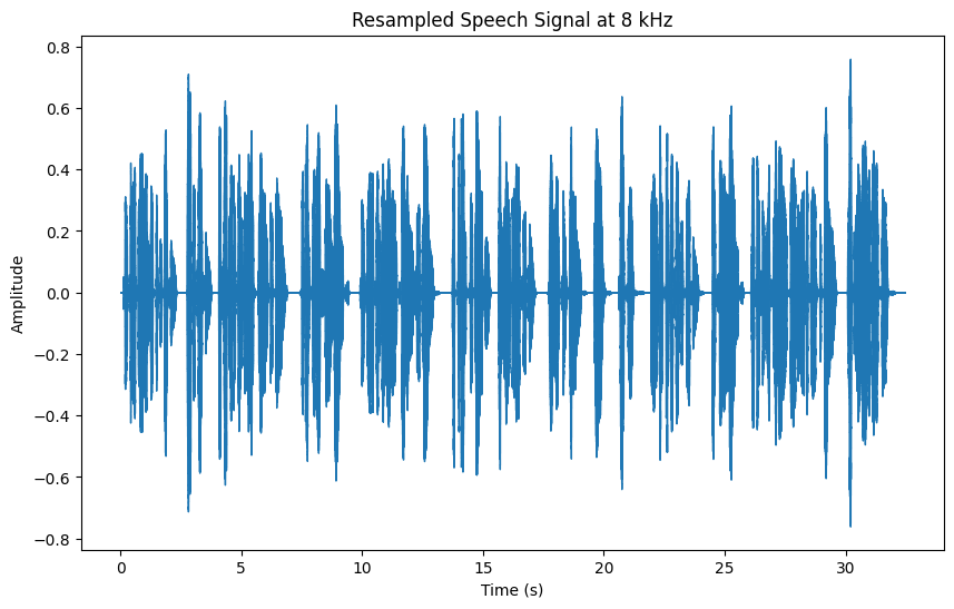
When you lower the sampling rate, you lose finer details of the speech signal, which can lead to aliasing and a reduction in sound quality. This highlights the importance of selecting an appropriate sampling rate.

1. Waveforms Don't Show Frequency Information Clearly

A waveform (librosa.display.waveshow()) mainly shows amplitude variations over time, but aliasing and loss of frequency details due to downsampling are not easily visible.
Even if you resample from 44.1 kHz to 8 kHz, the overall waveform shape remains similar unless the resolution is significantly degraded.

2. Resampling Affects High Frequencies More

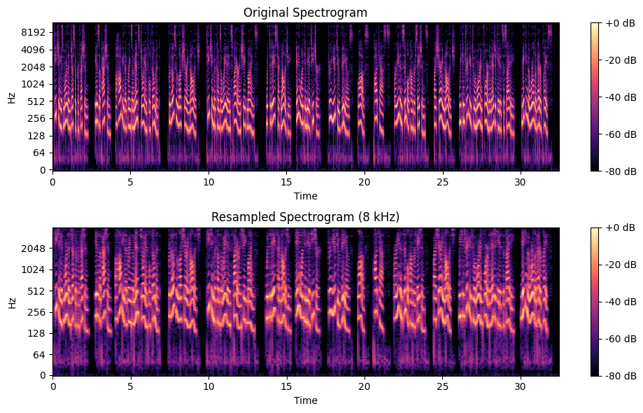
When you downsample, the higher frequencies (above half the new sampling rate) are removed due to the Nyquist theorem.
If you originally had a sampling rate of 44.1 kHz, the highest frequency component was 22.05 kHz. After resampling to 8 kHz, only frequencies below 4 kHz remain.
However, a waveform plot does not explicitly show frequency content.

Instead of plotting waveform, use spectrogram which reveal frequency components over time. A spectrogram is a visual representation of the frequency content of a signal over time. It displays time on the x-axis, frequency on the y-axis, and amplitude (intensity) as color or shading. Spectrograms are widely used in speech and audio processing to analyze sound characteristics, detect patterns, and observe changes in frequency components. Unlike waveform plots, which only show amplitude variations, spectrograms reveal important details such as pitch, harmonics, and noise, making them essential for tasks like speech recognition, speaker identification, and music analysis.

import librosa
import librosa.display
import matplotlib.pyplot as plt
import numpy as np
import librosa

# Load and resample audio
y, sr = librosa.load("shortaudio.wav", sr=None)
y_resampled = librosa.resample(y, orig_sr=sr, target_sr=8000)

# Compute spectrograms
D_orig = librosa.amplitude_to_db(np.abs(librosa.stft(y)), ref=np.max)
D_resampled = librosa.amplitude_to_db(np.abs(librosa.stft(y_resampled)), ref=np.max)

# Plot both spectrograms in one figure
plt.figure(figsize=(10, 6))

plt.subplot(2, 1, 1)
librosa.display.specshow(D_orig, sr=sr, x_axis="time", y_axis="log")
plt.colorbar(format="%+2.0f dB")
plt.title("Original Spectrogram")

plt.subplot(2, 1, 2)
librosa.display.specshow(D_resampled, sr=8000, x_axis="time", y_axis="log")
plt.colorbar(format="%+2.0f dB")
plt.title("Resampled Spectrogram (8 kHz)")

plt.tight_layout()
plt.show()

4. Quantization

Quantization is the process of mapping the continuous amplitude values of a signal to discrete values. This process is necessary because, in digital systems, we can't store continuous values — only discrete ones.

The bit-depth of a system determines the number of possible amplitude levels. Higher bit-depth results in more precise quantization, while lower bit-depth introduces more quantization noise. The most common bit-depths used in speech processing are 16-bit (CD quality) and 8-bit (low-quality audio).

Effect of Quantization:

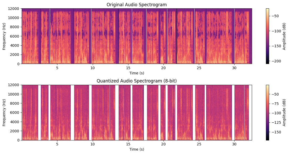
To understand how quantization affects speech, we can simulate this process by reducing the bit-depth. As the bit-depth decreases, we introduce more noise into the signal, which results in a loss of fidelity.

Here’s how to visualize the effect of quantization:

import numpy as np
import matplotlib.pyplot as plt
import soundfile as sf
import librosa
import librosa.display

# Load an audio file
audio, sr = librosa.load("example_audio.wav")

# Function to apply quantization
def quantize_signal(signal, num_bits):
    num_levels = 2 ** num_bits  # Quantization levels
    quantized_signal = np.round(signal * (num_levels / 2)) / (num_levels / 2)
    return quantized_signal

# Apply quantization (Example: 4-bit)
num_bits = 8
quantized_audio = quantize_signal(audio, num_bits)

# Save quantized audio
sf.write("quantized_example.wav", quantized_audio, sr)

# Plot Spectrograms Side by Side
plt.figure(figsize=(12, 6))

# Original Audio Spectrogram
plt.subplot(2, 1, 1)
plt.specgram(audio, Fs=sr, NFFT=1024, cmap="magma")
plt.title("Original Audio Spectrogram")
plt.xlabel("Time (s)")
plt.ylabel("Frequency (Hz)")
plt.colorbar(label="Amplitude (dB)")

# Quantized Audio Spectrogram
plt.subplot(2, 1, 2)
plt.specgram(quantized_audio, Fs=sr, NFFT=1024, cmap="magma")
plt.title(f"Quantized Audio Spectrogram ({num_bits}-bit)")
plt.xlabel("Time (s)")
plt.ylabel("Frequency (Hz)")
plt.colorbar(label="Amplitude (dB)")

plt.tight_layout()
plt.show()

When you reduce the bit-depth, you’ll notice more roughness in the waveform, which is the quantization noise. This is why higher bit-depths are used in professional audio systems to maintain a high-quality signal.

5. Conclusion

By understanding waveforms, sampling, and quantization, we gain a deeper appreciation for how speech signals are represented digitally. These concepts are crucial for various tasks in speech processing, such as Automatic Speech Recognition (ASR), speech synthesis, and audio compression.

Each step in the digitalization process — from capturing the waveform to quantizing the signal — has its own trade-offs in terms of quality and data size. By mastering these fundamental techniques, you can gain insights into how modern systems process and analyze speech.

Speech Signal Basics: Key Concepts of Waveforms, Sampling, and Quantization