Implementing LSTM RNN using Keras and TensorFlow

In this Article we will implement LTSM RNN model using Keras and TensorFlow. LSTM model was discussed in my previous article , but we will make this implementation easier by using Keras framework.

We will be using Jena Climate dataset recorded by the Max Planck Institute for Biogeochemistry. The dataset consists of 14 features such as temperature, pressure, humidity etc, recorded once per 10 minutes.

Lets Load the libraries

from urllib.request import urlretrieve
import numpy as np
import os
from tensorflow import keras

Load the Data

url=("https://s3.amazonaws.com/keras-datasets/jena_climate_2009_2016.csv.zip")
filename = "jena_climate_2009_2016.csv.zip"
path, headers = urlretrieve(url, filename)

Lets inspect the data

fname = os.path.join("jena_climate_2009_2016.csv")
with open(fname) as f:
    data = f.read()
lines = data.split("\n")
header = lines[0].split(",")
lines = lines[1:]
print(header)
print(len(lines))

['"Date Time"', '"p (mbar)"', '"T (degC)"', '"Tpot (K)"', '"Tdew (degC)"', '"rh (%)"', '"VPmax (mbar)"', '"VPact (mbar)"', '"VPdef (mbar)"', '"sh (g/kg)"', '"H2OC (mmol/mol)"', '"rho (g/m**3)"', '"wv (m/s)"', '"max. wv (m/s)"', '"wd (deg)"']
420451

We will Split the data into two numpy arrays as temperature and raw_data

temperature = np.zeros((len(lines),))
raw_data = np.zeros((len(lines), len(header) - 1))
for i, line in enumerate(lines):
    values = [float(x) for x in line.split(",")[1:]]
    temperature[i] = values[1]
    raw_data[i, :] = values[:]

Shape of the raw_data is

raw_data.shape
(420451, 14)

So we have 420451 samples containing 14 features of data

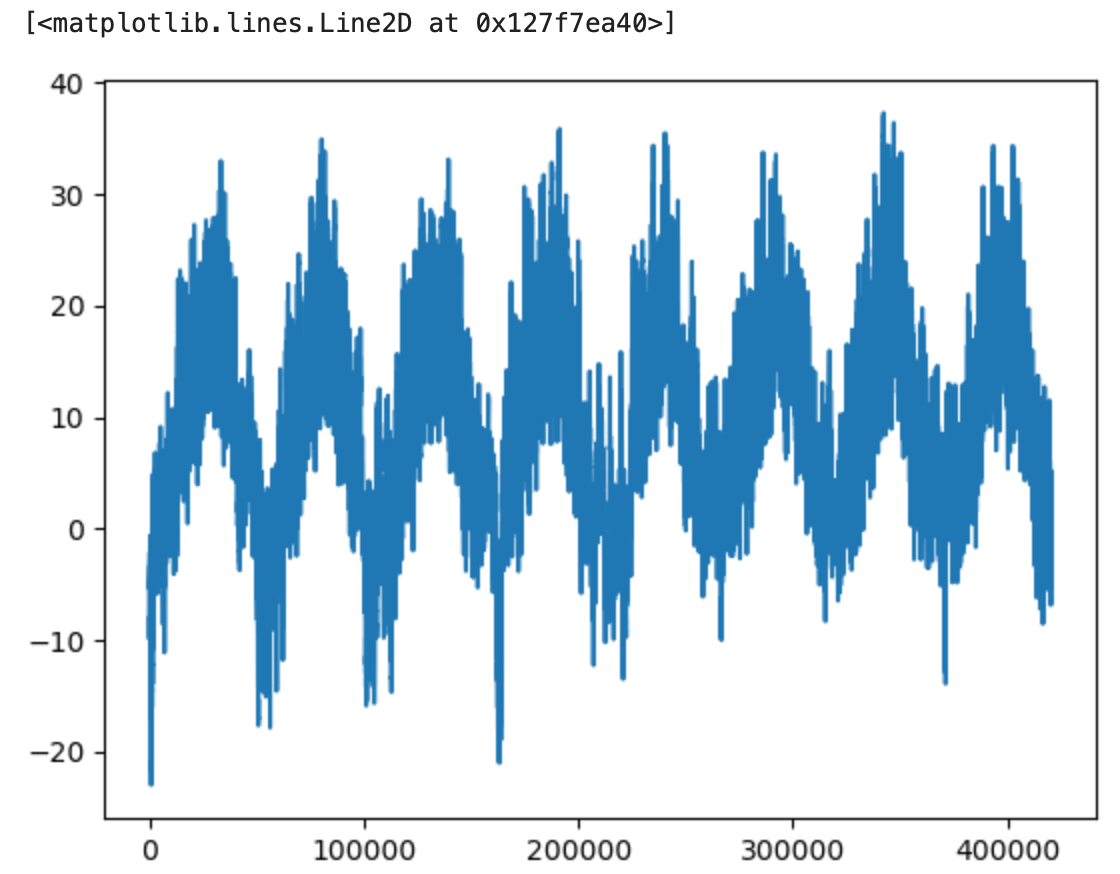
Plotting the temperature timeseries

from matplotlib import pyplot as plt
plt.plot(range(len(temperature)), temperature)

Computing the number of samples we'll use for each data split

We will split data into 50 % for training data, 25 % validation and test data each.

num_train_samples = int(0.5 * len(raw_data))
num_val_samples = int(0.25 * len(raw_data))
num_test_samples = len(raw_data) - num_train_samples - num_val_samples
print("num_train_samples:", num_train_samples)
print("num_val_samples:", num_val_samples)
print("num_test_samples:", num_test_samples)
print("raw_data Shape:", raw_data.shape)

num_train_samples: 210225
num_val_samples: 105112
num_test_samples: 105114
raw_data Shape: (420451, 14)

Normalizing the data

We will normalize the data using mean and standard deviation

mean = raw_data[:num_train_samples].mean(axis=0)
raw_data -= mean
std = raw_data[:num_train_samples].std(axis=0)
raw_data /= std

We will create Timeseries dataser by using keras API keras.utils.timeseries_dataset_from_array

We will keep the sequence length of 120 hr and use batch size of 256 form the samples. We will forecast temperature for the next 24 hr.

Instantiating datasets for training, validation, and testing

sampling_rate = 6
sequence_length = 120
delay = sampling_rate * (sequence_length + 24 - 1)
batch_size = 256

train_dataset = keras.utils.timeseries_dataset_from_array(
    raw_data[:-delay],
    targets=temperature[delay:],
    sampling_rate=sampling_rate,
    sequence_length=sequence_length,
    shuffle=True,
    batch_size=batch_size,
    start_index=0,
    end_index=num_train_samples)
val_dataset = keras.utils.timeseries_dataset_from_array(
    raw_data[:-delay],
    targets=temperature[delay:],
    sampling_rate=sampling_rate,
    sequence_length=sequence_length,
    shuffle=True,
    batch_size=batch_size,
    start_index=num_train_samples,
    end_index=num_train_samples + num_val_samples)
test_dataset = keras.utils.timeseries_dataset_from_array(
    raw_data[:-delay],
    targets=temperature[delay:],
    sampling_rate=sampling_rate,
    sequence_length=sequence_length,
    shuffle=True,
    batch_size=batch_size,
    start_index=num_train_samples + num_val_samples)

Inspecting the output of one of our datasets

for samples, targets in train_dataset:
    print("samples shape:", samples.shape)
    print("targets shape:", targets.shape)
    break

samples shape: (256, 120, 14)
targets shape: (256,)

Lets create A recurrent layer in Keras

Training and evaluating a dropout-regularized LSTM

inputs = keras.Input(shape=(sequence_length, raw_data.shape[-1]))
x = layers.LSTM(32, recurrent_dropout=0.25)(inputs)
x = layers.Dropout(0.5)(x)
outputs = layers.Dense(1)(x)
model = keras.Model(inputs, outputs)

callbacks = [
    keras.callbacks.ModelCheckpoint("jena_lstm_dropout.sample",
                                    save_best_only=True)
]
model.compile(optimizer="rmsprop", loss="mse", metrics=["mae"])
history = model.fit(train_dataset,
                    epochs=50,
                    validation_data=val_dataset,
                    callbacks=callbacks)

Epoch 48/50
819/819 [==============================] - 66s 80ms/step - loss: 8.9161 - mae: 2.3114 - val_loss: 11.4386 - val_mae: 2.6123
Epoch 49/50
819/819 [==============================] - 68s 83ms/step - loss: 8.8472 - mae: 2.3058 - val_loss: 11.4213 - val_mae: 2.6145
Epoch 50/50
819/819 [==============================] - 65s 79ms/step - loss: 8.8340 - mae: 2.3063 - val_loss: 11.3844 - val_mae: 2.6109

Load the the best saved model

model = keras.models.load_model("jena_lstm_dropout.sample")
print(f"Test MAE: {model.evaluate(test_dataset)[1]:.2f}")

405/405 [==============================] - 6s 14ms/step - loss: 10.3629 - mae: 2.5492
Test MAE: 2.55

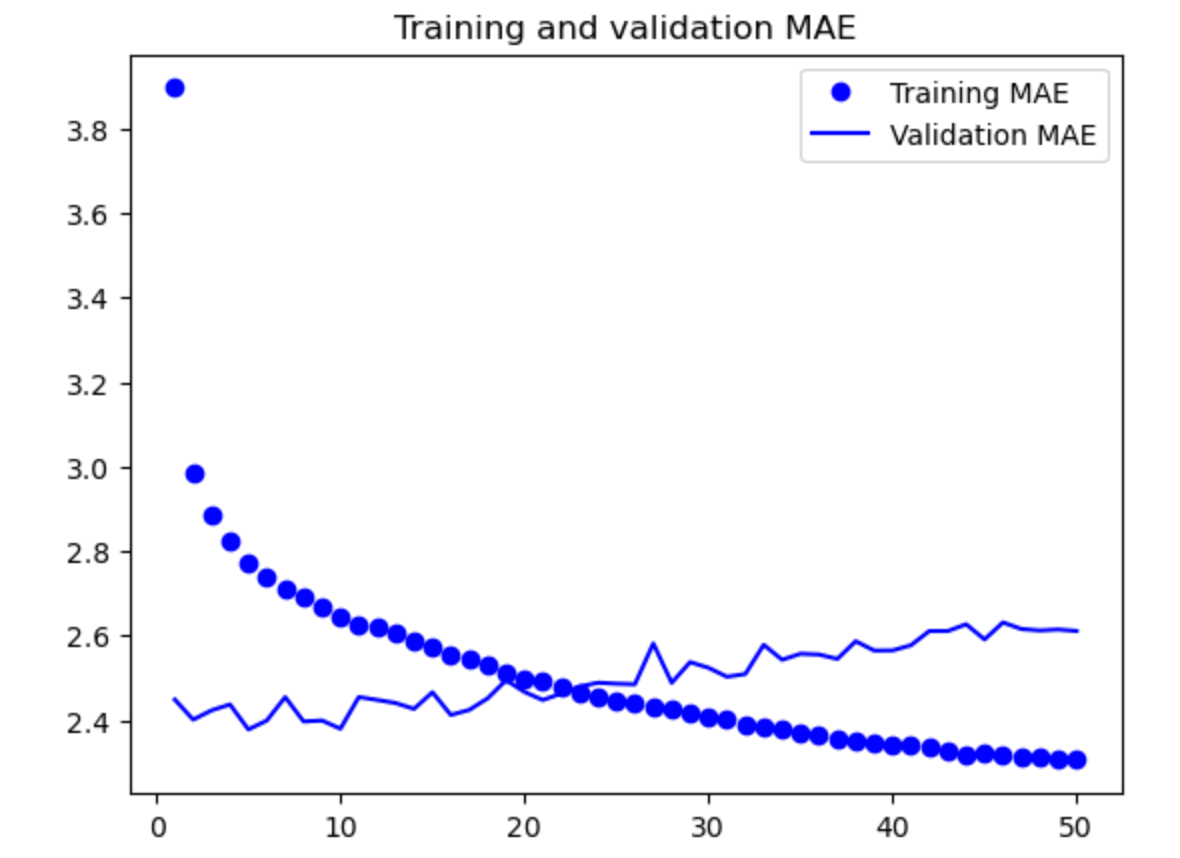
Lets plot

import matplotlib.pyplot as plt
loss = history.history["mae"]
val_loss = history.history["val_mae"]
epochs = range(1, len(loss) + 1)
plt.figure()
plt.plot(epochs, loss, "bo", label="Training MAE")
plt.plot(epochs, val_loss, "b", label="Validation MAE")
plt.title("Training and validation MAE")
plt.legend()
plt.show()