Hi there! 👋

I’m Dhyuthidhar, and if you’re new here, welcome! I love exploring computer science topics, especially machine learning, and breaking them down into easy-to-understand concepts. Today, let’s continue to talk about logistic regression.

In the last blog, I explained some functions that are useful to develop logistic regression code; now let me continue to explain the additional components that are used.

So in the last blog, the last function that I explained is forward and backward propagation, which returns the grads and costs.

As we got the gradients and cost function value, the next step is to optimize the values of the parameters W (weights) and b (bias).

Optimization

Write down the optimization function. The goal is to learn w and b by minimizing the cost function J.

For the parameter theta, the update rule is

$$\theta = \theta - \alpha \text{ } d\theta$$

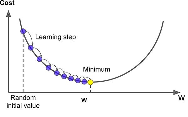
• Alpha represents the learning rate, a crucial concept in Gradient Descent, which helps optimize the cost function using parameters w and b.

• In the 2D graph of Gradient Descent, the goal is to reach the global minimum (the lowest point). To achieve this, the learning rate (alpha) guides the transition from a randomly initialized point to the global minimum. Essentially, alpha determines the size of each step taken toward the global minimum.

Instead of theta, we can put our two parameters W and b.

def optimize(w, b, X, Y, num_iterations=100, learning_rate=0.009, print_cost=False):

    w = w.copy()
    b = float(b)

    costs = []

    for i in range(num_iterations):
        # Cost and gradient calculation
        grads, cost = propagate(w, b, X, Y)

        # Retrieve derivatives from grads
        dw = grads["dw"]
        db = grads["db"]

        # Update rule
        w = w - learning_rate * dw
        b = b - learning_rate * db

        # Record the costs
        # For every 100 iterations we will record the cost instead of recording for every single iterations
        if i % 100 == 0:
            costs.append(cost)

            # Print the cost every 100 training iterations
            if print_cost:
                print(f"Cost after iteration {i}: {cost}")

    params = {"w": w,
              "b": b}

    grads = {"dw": dw,
             "db": db}

    return params, grads, costs

• We are going to iterate up to the number of iterations, which is a hyperparameter taken as an argument for the function.

• We will get the grads and cost values from the propagate function. Now we will grab them in the dw and db variables and update those values.

• For every 100 iterations we will print the cost.

• Then we will return the updated parameters, grads and costs with this function.

• The dw and db are used in gradient descent to show in which direction the point should flow so that we get to the global minima.

• You might encounter these questions while learning:

  In the first rule, you mentioned that we wouldn’t use any for loops, so why was one used here? While avoiding for loops is a common optimization in ML model development, they are sometimes necessary for iterating and running data multiple times through the model. As a result, you’ll notice there’s only one for loop in the entire code.

Prediction

The previous function will output the learned w and b. We will use w and b to predict the labels for a dataset X. Implement the predict() function. There are two steps to computing predictions:

1. Calculate Activation function

2. Convert the entries of a into 0 (if activation <= 0.5) or 1 (if activation > 0.5), and store the predictions in a vector Y_prediction If you wish, you can use an if/else statement in a for loop (though there is also a way to vectorize this).

def predict(w, b, X):

    m = X.shape[1] # No of training examples
    Y_prediction = np.zeros((1, m))
    w = w.reshape(X.shape[0], 1)

    # Compute probabilities
    A = sigmoid(np.dot(w.T, X) + b)

    # Convert probabilities to 0/1 predictions
    # you can either use Z.shape[1] in place of A as both have same shapes but you need to initialize or take Z as the parameter of the function
    for i in range(A.shape[1]):
        if A[0, i] > 0.5:
            Y_prediction[0, i] = 1
        else:
            Y_prediction[0, i] = 0

    return Y_prediction

• We initialized Y_prediction to zeros in the first line because it can make the process simple.

• In the second line, we ensure that w has the shape;(dim, 1) if it doesn't, we reshape it accordingly.

• We are initializing the activation function.

• Iterate through the activation function values for each example and update the Y_prediction based on the defined threshold of 0.5. You can relate to this part of code if you see the graph of the sigmoid function, which I explained in the previous blog.

• We will return Y_prediction using this function.

• If you guys have any questions, comment down! 👇

Now we need to use all these functions and develop a code for the model and run it in the main function.

Merge all functions into a model

You will now see how the overall model is structured by putting together all the building blocks (functions implemented in the previous parts) together in the right order.

model

Implement the model function. Use the following notation:

• Y_prediction_test for your predictions on the test set.

• Y_prediction_train for your predictions on the train set.

• parameters, grads, costs for the outputs of optimize()

def model(X_train, Y_train, X_test, Y_test, num_iterations=2000, learning_rate=0.5, print_cost=False):

    # Initialize parameters
    w, b = initialize_with_zeros(X_train.shape[0])

    # Gradient descent
    parameters, grads, costs = optimize(w, b, X_train, Y_train, num_iterations, learning_rate, print_cost)

    # Retrieve parameters w and b from dictionary "parameters"
    w = parameters["w"]
    b = parameters["b"]

    # Predict test/train set examples
    Y_prediction_test = predict(w, b, X_test)
    Y_prediction_train = predict(w, b, X_train)

    # Print train/test errors
    train_accuracy = 100 - np.mean(np.abs(Y_prediction_train - Y_train)) * 100
    test_accuracy = 100 - np.mean(np.abs(Y_prediction_test - Y_test)) * 100

    print(f"Train accuracy: {train_accuracy:.2f}%")
    print(f"Test accuracy: {test_accuracy:.2f}%")

    d = {
        "costs": costs,
        "Y_prediction_test": Y_prediction_test,
        "Y_prediction_train": Y_prediction_train,
        "w": w,
        "b": b,
        "learning_rate": learning_rate,
        "num_iterations": num_iterations
    }

    return d

• This is the whole development of the logistic regression using all the functions which we implemented till now.

• So first we will initialize the values of w and b as 0’s using the initialize_with_zeros() function.

• Then we will take values of parameters, cost, and grads from the optimize() function.

• Then we will update the parameters w and b.

• Then we will predict the values of Y_prediction_test and Y_prediction_trainusing the predict() function.

• Determine the accuracy of test and train predictions by calculating the difference between the two predicted and true values, then multiply the result by 100 to express it as a percentage.

• We are returning all the values as a dictionary because it will be flexible to use in the future code.

Testing Online Image

def test_with_online_image(url, model_dict, shape):

    response = requests.get(url)
    img = Image.open(BytesIO(response.content))
    img = img.resize((8, 8)).convert('L')  # Resize to 8x8 and grayscale

    # Convert to numpy array and flatten
    img_array = np.array(img).flatten() / 255.0

    # Reshape to match the model's expected input shape
    img_array = img_array.reshape(-1, 1) # converting into column vector

    # Make prediction
    prediction = predict(model_dict["w"], model_dict["b"], img_array)

    return int(prediction[0, 0])

• We are going to take the URL of the image as the argument and then use the dictionary, which contains the model parameters, and then we will reshape the image into the expected input shape.

• At the end, the prediction is returned as an integer. The predict() function outputs an array with the shape (1, m). By accessing prediction[0, 0] we extract the single value from this 2D array, and the int() function converts it from a NumPy integer type to a standard Python integer.

Main Function

def main():
    # Load dataset
    X_train, y_train, X_test, y_test, classes = load_basic_dataset()

    print(f"X_train shape: {X_train.shape}")
    print(f"y_train shape: {y_train.shape}")
    print(f"X_test shape: {X_test.shape}")
    print(f"y_test shape: {y_test.shape}")

    # Display a training example
    if X_train.shape[1] > 0:
        display_example(X_train, y_train, 0, "Training Example")

    # Train logistic regression model
    logistic_regression_model = model(
        X_train, y_train, X_test, y_test,
        num_iterations=2000, learning_rate=0.1, print_cost=True
    )

    # Plot learning curve
    costs = np.squeeze(logistic_regression_model['costs'])
    plt.figure(figsize=(10, 6))
    plt.plot(costs)
    plt.ylabel('cost')
    plt.xlabel('iterations (per hundreds)')
    plt.title(f"Learning rate = {logistic_regression_model['learning_rate']}")
    plt.show()

    # Try different learning rates
    learning_rates = [0.5, 0.1, 0.01]
    models = {}

    plt.figure(figsize=(10, 6))

    for lr in learning_rates:
        print(f"Training a model with learning rate: {lr}")
        models[str(lr)] = model(
            X_train, y_train, X_test, y_test,
            num_iterations=1500, learning_rate=lr, print_cost=False
        )
        print('\n' + "-------------------------------------------------------" + '\n')

        # Plot cost
        plt.plot(np.squeeze(models[str(lr)]["costs"]), label=str(models[str(lr)]["learning_rate"]))

    plt.ylabel('cost')
    plt.xlabel('iterations (hundreds)')
    plt.legend(loc='upper center')
    plt.show()

    # Display some test examples with predictions
    for i in range(min(5, X_test.shape[1])):
        # Get example and prediction
        example = X_test[:, i].reshape(8, 8)
        prediction = logistic_regression_model["Y_prediction_test"][0, i]
        true_label = y_test[0, i]

        # Display
        plt.figure(figsize=(4, 4))
        plt.imshow(example, cmap='gray')
        plt.title(f"True: {int(true_label)}, Predicted: {int(prediction)}")
        plt.axis('off')
        plt.show()

if __name__ == "__main__":
    main()

• The main function integrates all the implemented functions to generate a final prediction and visualization.

• First, the data is imported using the load_basic_dataset() function, splitting it into training and testing datasets along with their labels.

• Next, the shapes of the training and testing datasets are printed.

• A sample training image is then selected and plotted for visualization.

• Subsequently, the logistic regression model is initialized, which returns a dictionary containing the model parameters.

• The model is trained for 1500 iterations, with the cost being printed every 100 iterations.

• Cost vs. iteration graphs are plotted for each specified learning rate to analyze performance.

• As we can see from the learning curves above, the choice of learning rate significantly impacts model training. The learning rate of 0.1 offers an optimal balance between convergence speed and stability. With a learning rate of 0.5, the model converges faster initially but risks overshooting the minimum, potentially leading to less precise parameter values. Conversely, a learning rate of 0.01 shows more stable but much slower convergence, requiring many more iterations to reach the optimal values.

• This is why we typically use 0.1 as our default learning rate for this model - it provides fast convergence while maintaining sufficient precision in finding the optimal parameter values.

• Finally, for four selected examples, the images are plotted alongside their predicted values and corresponding true labels for comparison.

Conclusion

I have provided a mathematical explanation of the Logistic Regression model from the ground up. This will help you understand how it works, which is beneficial for learning deep learning as well. Additionally, you can explore its implementation using online visual references.

If you have any doubts, Comment below!✨👇

I will try to answer those questions.

I hope you understood the whole process, and now you can get the clarity in the below summary, which I posted in the previous blog:

References

These are the references that will be helpful to get to know more about this concept:

1. Here is the code: https://github.com/Dhyuthidhar2404/personal_blog/blob/main/Logistic_Practice.ipynb

2. Deep Learning or Machine Learning course by Andrew Ng in Coursera.

3. The 100 Pages of ML book by Andriy Burkov

4. Logistic Regression Code Introduction Part-1 blog

These two are wonderful resources to learn these concepts.

Action Step:

Try tracking these calculations for a few iterations with a different tiny image, like:

[16 0]
[16 0]

This could represent a vertical line on the left.

With label y = 0 (not a digit 1), follow the same steps and see how the model learns to classify it correctly.

You can practice the concept on paper.

Why I Share This

Simon Squibb believes that the best way to share knowledge is to make it simple and accessible. That’s exactly what I do—I break down complex technology into something easy and exciting.

Tech should inspire you, not intimidate you.

Imagine a world without machine learning—every company would need to manually analyze massive datasets just to extract insights. Deep learning changed that game. It enables anyone with data to uncover patterns and build intelligent systems without relying solely on traditional methods.

I share knowledge this way because I want you to feel that excitement too.

If this post made you think differently about tech, check out my other blogs. Let’s make tech easy and exciting—together! 🚀