Speech processing is a critical part of AI and Audio Technologies. In this article, we’ll explore fundamental techniques used for speech feature extraction:

Fourier Transform & Spectrograms (Visualizing speech in the frequency domain)
Mel-Frequency Cepstral Coefficients (MFCCs) (Key features for human speech signal)

1️⃣ Fourier Transform & Spectrograms

What is the Fourier Transform?

Sound waves are typically represented in the time domain (waveforms), but analyzing their frequency components is crucial. The Fourier Transform (FT) converts a time-domain signal into its frequency components.

The Short-Time Fourier Transform (STFT) is commonly used in speech processing to create spectrograms, which display how frequencies change over time.

Spectrograms

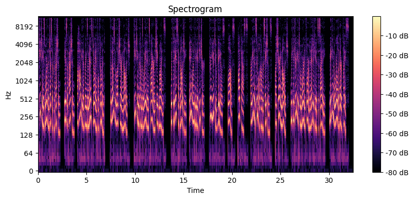
A spectrogram is a visual representation of sound frequencies of a signal as it varies with time. Unlike waveforms that show amplitude over time, spectrograms reveal the frequency content.

Types of Spectrograms

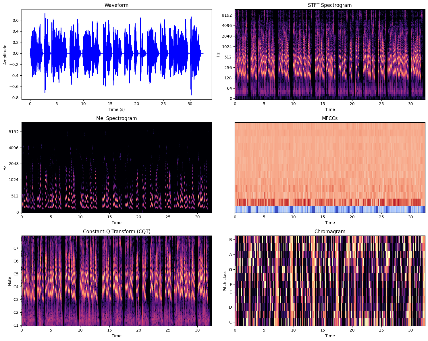
Short-Time Fourier Transform (STFT) Spectrogram – Standard time-frequency representation.
Log-Scaled Spectrogram – More interpretable for human perception.
Mel Spectrogram – Based on the Mel scale, which mimics human hearing.
MFCC Spectrogram – Compressed Mel spectrogram, commonly used in speech recognition.
CQT (Constant-Q Transform) Spectrogram – Good for musical applications.
Chromagram – Highlights pitch classes (useful in music & speech emotion detection).

🔹 How to generate a spectrogram in Python?

import librosa
import librosa.display
import numpy as np
import matplotlib.pyplot as plt

def plot_waveform_and_spectrograms(audio_path):
    # Load audio file
    y, sr = librosa.load(audio_path, sr=None)

    # Compute different spectrograms
    D = np.abs(librosa.stft(y))  # Short-Time Fourier Transform (STFT)
    D_db = librosa.amplitude_to_db(D, ref=np.max)  # Log-scale spectrogram

    mel_spectrogram = librosa.feature.melspectrogram(y=y, sr=sr, n_mels=128)
    mel_spectrogram_db = librosa.amplitude_to_db(mel_spectrogram, ref=np.max)

    mfccs = librosa.feature.mfcc(y=y, sr=sr, n_mfcc=13)

    cqt = np.abs(librosa.cqt(y, sr=sr, hop_length=512))
    cqt_db = librosa.amplitude_to_db(cqt, ref=np.max)

    chroma = librosa.feature.chroma_stft(y=y, sr=sr, hop_length=512)

    # Create subplots
    fig, ax = plt.subplots(3, 2, figsize=(15, 12))

    # Waveform
    ax[0, 0].plot(np.linspace(0, len(y) / sr, num=len(y)), y, color='b')
    ax[0, 0].set_title("Waveform")
    ax[0, 0].set_xlabel("Time (s)")
    ax[0, 0].set_ylabel("Amplitude")

    # STFT Spectrogram
    librosa.display.specshow(D_db, sr=sr, x_axis='time', y_axis='log', ax=ax[0, 1])
    ax[0, 1].set_title("STFT Spectrogram")

    # Mel Spectrogram
    librosa.display.specshow
        (mel_spectrogram_db, sr=sr, x_axis='time', y_axis='mel', ax=ax[1, 0])
    ax[1, 0].set_title("Mel Spectrogram")

    # MFCCs
    librosa.display.specshow(mfccs, sr=sr, x_axis='time', ax=ax[1, 1])
    ax[1, 1].set_title("MFCCs")

    # Constant-Q Transform (CQT)
    librosa.display.specshow(cqt_db, sr=sr, x_axis='time', y_axis='cqt_note', ax=ax[2, 0])
    ax[2, 0].set_title("Constant-Q Transform (CQT)")

    # Chromagram
    librosa.display.specshow(chroma, sr=sr, x_axis='time', y_axis='chroma', ax=ax[2, 1])
    ax[2, 1].set_title("Chromagram")

    plt.tight_layout()
    plt.show()

# Example Usage
audio_path = "audio.wav"  # Replace with your audio file
plot_waveform_and_spectrograms(audio_path)

🔍 How to Interpret a Spectrogram

A spectrogram is a 3D representation of an audio signal where:

X-axis (Time) → Represents time progression.
Y-axis (Frequency) → Shows different frequency components.
Color Intensity (Amplitude/Power) → Represents the energy (loudness) of each frequency at a given time.

import librosa
import librosa.display
import numpy as np
import matplotlib.pyplot as plt

# Load an audio file
y, sr = librosa.load("audio.wav", sr=None)

# Compute the Short-Time Fourier Transform (STFT)
D = librosa.amplitude_to_db(np.abs(librosa.stft(y)), ref=np.max)

# Display the Spectrogram
plt.figure(figsize=(10, 4))
librosa.display.specshow(D, sr=sr, x_axis='time', y_axis='log')
plt.colorbar(format='%+2.0f dB')
plt.title("Spectrogram")
plt.show()

📊 Example Spectrogram Interpretation

Scenario: Suppose you have a spectrogram of someone saying "Hello".

Low-frequency bands (below 300 Hz) → Represent voiced sounds (e.g., vowels like "e" in "hello").
Higher frequency components (above 3000 Hz) → Capture fricatives (e.g., "h" sound).
Vertical dark bands → Indicate plosive sounds (e.g., "h" in "hello").
Continuous smooth areas → Represent vowels, which have a longer duration.

📌 Observing Key Features

Formants: Dark horizontal bands that indicate resonant frequencies of speech sounds.
Harmonics: Parallel lines visible in periodic sounds like vowels.
Silences/Gaps: Flat regions without frequency content indicate pauses.

Example:
🚀 A word like "Hello" will have strong frequency energy at the start ("H"), followed by distinct formants for "e" and "o".

2️⃣ Mel-Frequency Cepstral Coefficients (MFCCs)

What are MFCCs?

MFCCs are widely used in speech recognition as they mimic how humans perceive sound. The human ear is more sensitive to certain frequencies, so MFCCs use a Mel scale to focus on perceptually important features. They represent the speech signal's spectral properties in a way that mimics human auditory perception.

Why are MFCCs Important?

The human ear is more sensitive to certain frequencies.
MFCCs use the Mel scale, which compresses high frequencies.
Unlike raw spectrograms, MFCCs capture speech-relevant information efficiently.

How MFCCs are Computed

Pre-emphasis – Boost high frequencies.
Framing – Divide speech into small time windows.
Windowing – Apply a Hamming window to reduce discontinuities.
FFT (Fast Fourier Transform) – Convert to the frequency domain.
Mel Filter Bank – Apply triangular filters to mimic human hearing.
Logarithm & Discrete Cosine Transform (DCT) – Extract compact feature vectors.

🔹 Extracting MFCCs using Librosa:

mfccs = librosa.feature.mfcc(y=y, sr=sr, n_mfcc=13)
plt.figure(figsize=(10, 4))
librosa.display.specshow(mfccs, sr=sr, x_axis='time')
plt.colorbar()
plt.title("MFCCs")
plt.show()

🔍 How to Interpret MFCCs

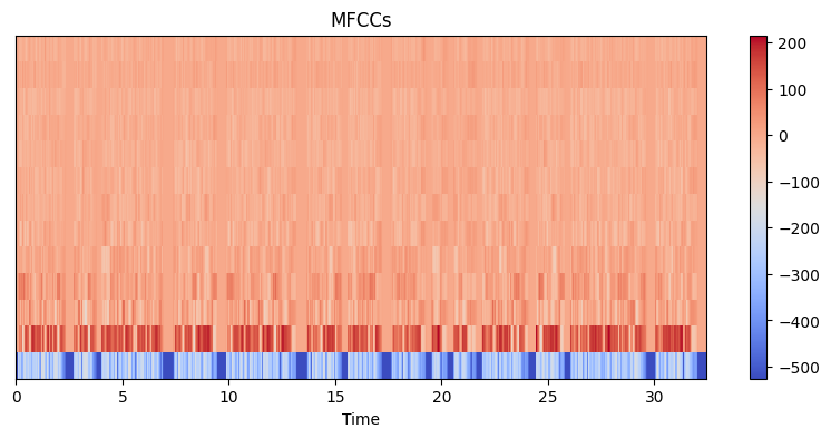
MFCCs are compact representations of the spectrogram, emphasizing speech-relevant features while ignoring unnecessary frequency information.

📊 Reading MFCCs

X-axis (Time): Shows the progression of speech over time.
Y-axis (MFCC Coefficients): Represents different frequency bands (similar to spectrogram frequency axis but compressed using the Mel scale).
Color Intensity: Represents energy in that frequency band.

📌 Understanding MFCC Components

Lower MFCCs (1-2): Represent the overall spectral shape (like pitch and loudness).
Middle MFCCs (3-8): Capture important phoneme information (helps in speech recognition).
Higher MFCCs (9+): Represent fine spectral details, which are often ignored in ASR models.

📌 Key Observations

Different words produce different MFCC patterns.
- Vowel sounds → Show stable, smooth coefficient variations.
- Consonants → Produce sharper changes.
- Fricatives (like “s” or “sh”) → Appear as high-frequency variations.
MFCCs are useful for distinguishing speakers and speech emotions.
- Different speakers will have slightly different MFCC patterns due to vocal tract differences.
- Emotions affect energy distribution, leading to varying MFCC patterns.

3️⃣🎯 Conclusion

The Fourier Transform helps analyze frequencies in speech.
Spectrograms visualize how frequencies change over time.
MFCCs are key features for human speech models.

Understanding Speech Features: Fourier Transform, Spectrograms, and MFCCs