Forward Pass of CNN

Last time we had an overview of the architecture of CNN, its components and some terminologies related to it. In this article, we will understand the working of the forward pass of a CNN from a mathematical viewpoint.

We will follow the journey of a single image matrix and observe how it changes throughout the pipeline. For this demonstration we will have only a single convolution layer and max pool layer, and we will consider the image to be single-channelled for simplicity.

Convolutional layer

Do you remember what we did in convolution last time? We flipped the second array and multiplied and added corresponding values while treating the second array like a sliding window. Let’s apply the same procedure to 2D matrices.

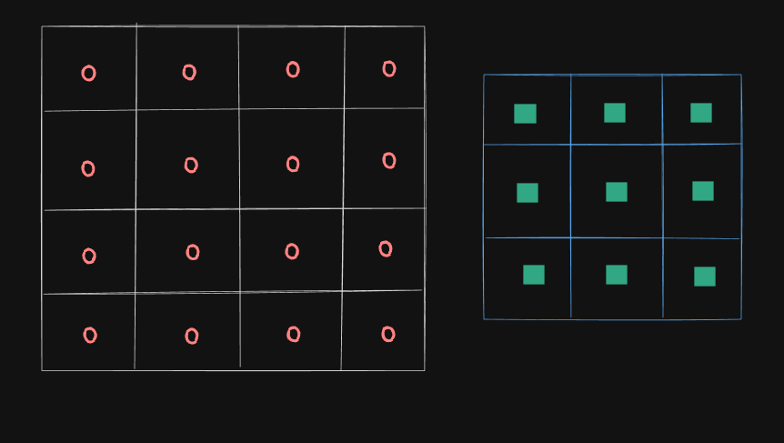
For demonstration, we will take a 4 x 4 image matrix with the numbers inside it represented by a red circle and a 3 x 3 kernel with its numbers represented by a square.

(Note: The pixel values are not necessarily same, its just a way of representation.)

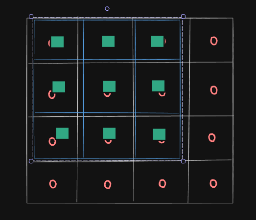
Firstly, we will overlap the kernel with the upper-left portion of the image matrix. Then the corresponding numbers will be multiplied and added to give one resultant. As you can see, this process will be repeated 3 more times, resulting in a 2 x 2 matrix.

You can extend this process for a 5X5 matrix as well, in which case we will get a 3X3 resultant matrix. So from this, we can generalise a formula:

For a convolution between n X n image matrix and a f X f filter, we will get a (n - f + 1) x (n - f + 1) sized resultant matrix.

Note: We did not explicitly flipped any matrix this time. That is because it is a redundant step and we will compensate for its purpose through backpropagation which we will see later.

Padding

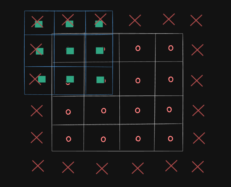
You might’ve noticed a flaw in the above process. All pixels are not being treated the same way. The pixels on left and right edges are interacting with the filter only once, while those in the centre are interacting all four times. Clearly, this will result in incorrect biases.

To fix this, we use padding. We add a row of zeros surrounding the image matrix. They will handle the hanging portion of the filter and we will be able to inculcate the corner and edge pixels more than once. For padding of 1 the image size will increase by 2 in both dimensions.

This also allows us to maintain the size of the resultant feature map to be same as that of the image. To do that, we have to carefully select the optimum padding size, the formula for which is:

$$p = \frac{(f-1)}{2}$$

Stride

The number of columns(or rows) our window slides through at a time is called stride. In all the above examples, the stride was one. Can you imagine what would happen if the stride was 2 in the above example?

The number of times we do convolution is reduced to only 4, similar to the very first example.

After accounting for stride and padding, our formula for final size of the feature map becomes :

$$W_f = \frac{W_i - f + 2P}{S} + 1$$

where W_i is the size of the image matrix and W_f is the size of the feature map.

If you want these two sizes to be the same then the formula for padding can be becomes :

$$P = \frac{W_i(S-1) -S + f}{2}$$

Implementing Convolutional Layer

For now, we will take filter size and number of filters as parameters. CNNs generally take multiple filters, each for capturing different features of the image. Each will go through the whole process separately and the final output feature map will have depth equal to the number of filters.

Let’s first create a filter matrix filled with random numbers.

class ConvLayer:
    def __init__(self, num_filters, filter_size):
        self.num_filters = num_filters
        self.filter_size = filter_size
        self.filters = np.random.randn(num_filters, filter_size, filter_size) / 9

Now we need to create a function for sliding windows/kernels. For that we will use the formula we discussed above. We will extract the height and width of the image (which is same in most cases) and reduce it by the filter size then add 1. The only thing which might seem a bit new to some is the use of yield instead of return.

Other’s may have seen that before in generators in python.

We won’t go into the details here, but generators are like functions, only that they allow us to generate values on-the-fly instead of storing them somewhere. This saves memory overhead of calculating and storing different regions separately.

(To be honest this wasn’t my first thought either so don’t worry if this didn’t come intuitively to you).

def iterate_regions(self, image):
        h, w = image.shape
        for i in range(h - self.filter_size + 1):
            for j in range(w - self.filter_size + 1):
                region = image[i:(i + self.filter_size), j:(j + self.filter_size)]
                yield region, i, j

Rest is straightforward. We will create an zero matrix first for output. Then we use the generator to fetch the required region and convolve that region with our filters. We won’t be using any padding or strides for this demonstration to keep it as simple as possible.

def forward(self, input):
        self.input = input
        h, w = input.shape
        output = np.zeros((h - self.filter_size + 1, w - self.filter_size + 1, self.num_filters))

        for region, i, j in self.iterate_regions(input):
            output[i, j] = np.sum(region * self.filters, axis=(1, 2))

        return output

Max Pool Layer

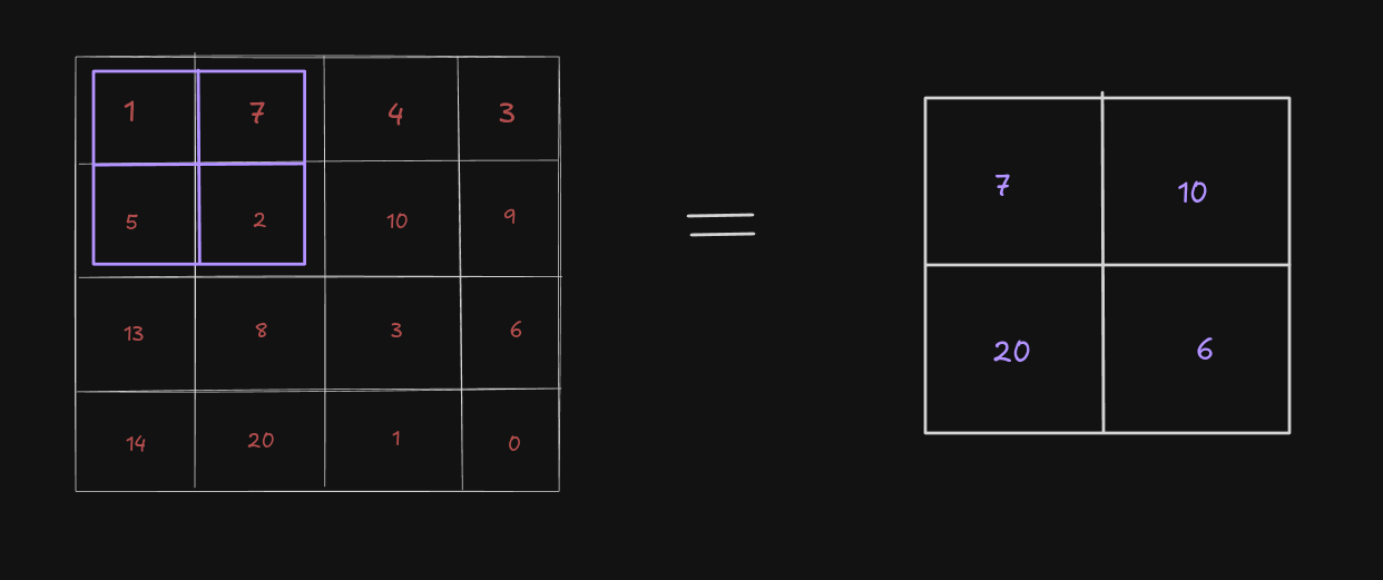
Max pooling is a down-sampling technique applied to feature maps. It operates by dividing the input feature map into non-overlapping or overlapping sub-regions (e.g., 2 x 2 or 3 x 3 grids) and selecting the maximum value within each sub-region.

For example, if we have a 4 x 4 feature map and a kernel of size 2 x 2 with stride 2, we will obtain a down-sampled output of 2 x 2 matrix with only the maximum value from each corresponding sub-grid.

Now that the theoretical part is done, let’s try to implement this stuff.

class MaxPoolLayer:
    def __init__(self, size=2):
        self.size = size

    def forward(self, input):
        self.input = input
        h,w, num_filters = input.shape
        output = np.zeros((h // self.size, w // self.size, num_filters))

        for i in range(0, h, self.size):
            for j in range(0, w, self.size):
                output[i // self.size, j // self.size] = np.amax(input[i:i+self.size, j:j+self.size], axis=(0, 1))

        return output

Activation Layer

We will be using ReLU Activation Layer, except for the final FC layer, where softmax must be used.

class ReLULayer:

    def forward(self, input):
        self.input = input
        return np.maximum(0, input)

Fully Connected Layer

This as said before, is similar to what you would see in regular Neural Networks. We have also done a separate blog on building them from scratch.

class FullyConnectedLayer:
    def __init__(self, input_size, num_classes):
        self.weights = np.random.randn(input_size, num_classes) / input_size
        self.biases = np.zeros(num_classes) 

    def forward(self, input):
        self.input = input  
        return np.dot(input, self.weights) + self.biases

Just remember that before using this, we will have to flatten the image.

For an image of size 28 × 28, the feature map will be of size 26 × 26 × 8 and after max pooling it will be of size 13 × 13 × 8 where 8 is the number of filters. After flattening it will become 1352 × 1.

This was the forward pass of our CNN. But this is just 45% of work. Rest is writing code for back-propagation and setting up the complete pipeline.