Backward Pass of CNN

Since the forward pass ended on the Fully Connected Layer, it is only natural to begin the discussion of backpropagation from that layer.

Fortunately for us, it is not any different than what we usually see in regular Neural Networks. Therefore, we can just proceed to implement it:

class FullyConnectedLayer:
    def __init__(self, input_size, num_classes, lr=0.01):
        self.weights = np.random.randn(input_size, num_classes) / input_size
        self.biases = np.zeros(num_classes)
        self.lr = lr  

    def forward(self, input):
        self.input = input  
        return np.dot(input, self.weights) + self.biases

    def backward(self, dL_dout):
        dL_dB = dL_dout.sum(axis = 0)
        dL_dW = self.input.reshape(1352, 1) @ dL_dout.reshape(1, 10) #for single image

        dL_dinput = np.dot(dL_dout, self.weights.T)

        self.weights -= self.lr*dL_dW
        self.biases -= self.lr*dL_dB
        return dL_dinput

Here, you might notice that instead of the dot product, we are using the matrix multiplication with reshape. This is because our example implementation is only for a single image and this reshaping helps us align the matrices correctly. We will have a look at a more general implementation in later parts of the series.

Max Pool Layer

Since in Max Pool Layer, only the maximum value is retained in the forward pass, so any change from the dL_dout will be passed only to that specific position which has the maximum value right now.

 def backward(self, dL_dout):

        dL_dinput = np.zeros(self.input.shape)
        h, w, num_filters = self.input.shape

        for i in range(0, h, self.size):
            for j in range(0, w, self.size):
                region = self.input[i:i+self.size, j:j+self.size]
                max_vals = np.amax(region, axis = (0,1))

                for k in range(num_filters):

                    for ii in range(self.size):
                        for jj in range(self.size):
                            if region[ii, jj, k] == max_vals[k]:
                                dL_dinput[i+ii, j+jj, k] = dL_dout[i // self.size, j // self.size, k]

        return dL_dinput

But if you combine this with our previous code for forward implementation you will see that it looks quite bulky and repetitive which is true since we are rewriting the code for finding the maximum element.

Instead what we can do is extract and store the indices of the maximum elements using np.argmax() function. But for that we will have to use a flat array and convert the indices back to the required shape using np.unravel_index. This is the final outlook.

class MaxPoolLayer:
    def __init__(self, size=2):
        self.size = size
        self.max_positions = None  #For storing the indices of max. values

    def forward(self, input):
        self.input = input
        h, w, num_filters = input.shape
        output = np.zeros((h // self.size, w // self.size, num_filters))
        self.max_positions = np.zeros((h // self.size, w // self.size, num_filters, 2), dtype=int)

        for i in range(0, h, self.size):
            for j in range(0, w, self.size):
                region = input[i:i+self.size, j:j+self.size]
                max_vals = np.amax(region, axis=(0, 1))
                output[i // self.size, j // self.size] = max_vals

                for k in range(num_filters):
                    max_pos = np.unravel_index(np.argmax(region[:, :, k]), (self.size, self.size))
                    self.max_positions[i // self.size, j // self.size, k] = (i + max_pos[0], j + max_pos[1])

        return output

    def backward(self, dL_dout):
        dL_dinput = np.zeros(self.input.shape)
        h_out, w_out, num_filters = dL_dout.shape

        for i in range(h_out):
            for j in range(w_out):
                for k in range(num_filters):
                    max_i, max_j = self.max_positions[i, j, k]
                    dL_dinput[max_i, max_j, k] = dL_dout[i, j, k]

        return dL_dinput

ReLU Layer

Again, the backpropagation in ReLU layer stays the same as that of ANN. The gradient from the upper layer is passed on as it is, but only to those indices where the value is positive.

def backward(self, dL_dout):

        dL_dinput = dL_dout.copy()
        dL_dinput[self.input <= 0] = 0  

        return dL_dinput

For Convolution layer

Here too, we already have the differential of Loss w.r.t the output (dL/d_out).

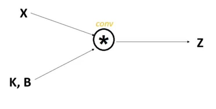
In this image, X represents the input, K is kernel which represents the weights which we will be updating, B is biases and Z represents the output. Now you might ask “Hey, we didn’t put any bias in our forward pass?” which is right, but for the sake of numerical derivation, let’s just assume for a second that we did.

This lays a nice carpet for us to tinker with, because this is similar to the picture of regular neural networks which we have worked with before. We have dL/dZ and we need to find dL/dK and dL/dB so that we can adjust the filters and biases through gradient descent.

For ease of calculation, we will use a 3 × 3 input matrix, and a 2 × 2 kernel, since the results we derive from these calculations will be standard.

Firstly, we have:

$$X \circledast K + B = Z$$

which means,

$$\begin{bmatrix} X_{11} & X_{12} & X_{13} \\ X_{21} & X_{22} & X_{23} \\ X_{31} & X_{32} & X_{33} \end{bmatrix} \circledast \begin{bmatrix} K_{11} & K_{12} \\ K_{21} & K_{22} \end{bmatrix} + B = \\ \begin{bmatrix} Z_{11} & Z_{12} \\ Z_{21} & Z_{22} \end{bmatrix}$$

which gives us 4 equations:

$$\begin{align} Z_{11} &= X_{11}K_{11} + X_{12}K_{12} + X_{21}K_{21} + X_{22}K_{22} + B \\ Z_{12} &= X_{12}K_{11} + X_{13}K_{12} + X_{22}K_{21} + X_{23}K_{22} + B \\ Z_{21} &= X_{21}K_{11} + X_{22}K_{12} + X_{31}K_{21} + X_{32}K_{22} + B \\ Z_{22} &= X_{22}K_{11} + X_{23}K_{12} + X_{32}K_{21} + X_{33}K_{22} + B \\ \end{align}$$

From chain rule, we know:

$$\frac{\partial L}{\partial K} = \frac{\partial L}{\partial Z}\cdot\frac{\partial Z}{\partial K}$$

But that was for single entities only. You can see that K is a kernel representing 4 different weights. So we will have to calculate the change in loss function w.r.t. weight for all 4 of them, which will make it look like this.

$$\frac{\partial L}{\partial K} = \begin{bmatrix} \frac{\partial L}{\partial k_{11}} & \frac{\partial L}{\partial k_{12}}\\ \frac{\partial L}{\partial k_{21}} & \frac{\partial L}{\partial k_{22}} \end{bmatrix}$$

Modifying the above equation:

$$\frac{\partial L}{\partial K_{mn}} = \frac{\partial L}{\partial Z}\cdot\frac{\partial Z}{\partial K_{mn}}$$

which if you think about it, seems incomplete or incorrect. That is because the output Z is also not a single entity.

While calculating the change in loss function w.r.t a particular weight, we will have to consider all those instances where any of the outputs is affected by that weight, because all of those outputs, in turn, will affect the loss function individually.

For example, for k_11 we will have:

$${\small \begin{align} \frac{\partial L}{\partial K_{11}} &= (\frac{\partial L}{\partial Z_{11}}\cdot\frac{\partial Z_{11}}{\partial K_{11}}) + (\frac{\partial L}{\partial Z_{12}}\cdot\frac{\partial Z_{12}}{\partial K_{11}}) + (\frac{\partial L}{\partial Z_{21}}\cdot\frac{\partial Z_{21}}{\partial K_{11}}) + (\frac{\partial L}{\partial Z_{22}}\cdot\frac{\partial Z_{22}}{\partial K_{11}}) \\ \\ \\ &= \sum_{j=1}^{W_{out}}\sum_{i=1}^{H_{out}} (\frac{\partial L}{\partial Z_{ij}}\cdot\frac{\partial Z_{ij}}{\partial K_{11}}) \end{align} }$$

where W_out and H_out are the width and height of the output window respectively. We can replace K_11 with K_mn to generalise the formula but before that,

We already have all the dL/dZ_ij terms, from the parameters we will take. What we need is the second term, which we can easily get from the four equations written above.

For k_11:

$$\begin{align} Z_{11} &= X_{11}K_{11} + X_{12}K_{21} + X_{21}K_{12} + X_{22}K_{22} + B \\ \\ \implies \frac{\partial Z_{11}}{\partial K_{11}} &= X_{11} \end{align}$$

which can be generalised for all other outputs as well. So:

$${\small \frac{\partial L}{\partial K_{11}} = (\frac{\partial L}{\partial Z_{11}}\cdot X_{11})+ (\frac{\partial L}{\partial Z_{12}}\cdot X_{12}) + (\frac{\partial L}{\partial Z_{21}}\cdot X_{21}) + (\frac{\partial L}{\partial Z_{22}}\cdot X_{22}) }$$

You can repeat the process to obtain similar results for the other three and this is what it will look like:

$${\small \begin{align} \frac{\partial L}{\partial K_{11}} &= (\frac{\partial L}{\partial Z_{11}}\cdot X_{11})+ (\frac{\partial L}{\partial Z_{12}}\cdot X_{12}) + (\frac{\partial L}{\partial Z_{21}}\cdot X_{21}) + (\frac{\partial L}{\partial Z_{22}}\cdot X_{22}) \\ \frac{\partial L}{\partial K_{12}} &= (\frac{\partial L}{\partial Z_{11}}\cdot X_{12})+ (\frac{\partial L}{\partial Z_{12}}\cdot X_{13}) + (\frac{\partial L}{\partial Z_{21}}\cdot X_{22}) + (\frac{\partial L}{\partial Z_{22}}\cdot X_{23}) \\ \frac{\partial L}{\partial K_{21}} &= (\frac{\partial L}{\partial Z_{11}}\cdot X_{21})+ (\frac{\partial L}{\partial Z_{12}}\cdot X_{22}) + (\frac{\partial L}{\partial Z_{21}}\cdot X_{31}) + (\frac{\partial L}{\partial Z_{22}}\cdot X_{32}) \\ \frac{\partial L}{\partial K_{22}} &= (\frac{\partial L}{\partial Z_{11}}\cdot X_{22})+ (\frac{\partial L}{\partial Z_{12}}\cdot X_{23}) + (\frac{\partial L}{\partial Z_{21}}\cdot X_{32}) + (\frac{\partial L}{\partial Z_{22}}\cdot X_{33}) \end{align} }$$

Seems overwhelming? How about this?

$$\begin{bmatrix} X_{11} & X_{12} & X_{13} \\ X_{21} & X_{22} & X_{23} \\ X_{31} & X_{32} & X_{33} \end{bmatrix} \circledast \begin{bmatrix} \frac{\partial L}{\partial Z_{11}} & \frac{\partial L}{\partial Z_{12}} \\ \frac{\partial L}{\partial Z_{21}} & \frac{\partial L}{\partial Z_{22}} \end{bmatrix} = \\ \begin{bmatrix} \frac{\partial L}{\partial K_{11}} & \frac{\partial L}{\partial K_{12}} \\ \frac{\partial L}{\partial K_{21}} & \frac{\partial L}{\partial K_{22}} \end{bmatrix}$$

Yes. The above four equations can be summarised with the use of a single convolution operation. If you look again at the equations, you will see that they are not much different from the initial four, just the positions of terms with K and terms with Z has been reversed through our logic. So it is natural for it to follow this pattern.

It can also be written as:

$$\frac{\partial L}{\partial K} = conv(X , \frac{\partial L}{\partial Z})$$

We can use the same equations to calculate the partial derivative w.r.t Biases as well and it will result in this:

$$\frac{\partial L}{\partial B} = sum(\frac{\partial L}{\partial Z})$$

This completes half of our work. The rest half is about calculating the change in loss w.r.t the input values. For that, again, we will use the same logic.

Find all those instances where the output is affected by that particular input, multiply the error signal with them and add. For example, let’s take X_11

$$\begin{align} \frac{\partial L}{\partial X_{11}} &= \frac{\partial L}{\partial Z_{11}}\cdot\frac{\partial Z_{11}}{\partial X_{11}} \\ \\ \implies \frac{\partial L}{\partial X_{11}} &= \frac{\partial L}{\partial Z_{11}}\cdot K_{11} \end{align}$$

because Z_11 is the only output which is being affected by the input X_11. But this isn’t the case with X_12. It affects both Z_11 and Z_12. Doing this, you will get these equations:

$${\small \begin{align} \frac{\partial L}{\partial X_{11}} &= (\frac{\partial L}{\partial Z_{11}}\cdot K_{11}) \\ \frac{\partial L}{\partial X_{12}} &= (\frac{\partial L}{\partial Z_{11}}\cdot K_{12}) + (\frac{\partial L}{\partial Z_{12}} \cdot K_{11}) \\ \frac{\partial L}{\partial X_{13}} &= (\frac{\partial L}{\partial Z_{12}}\cdot K_{12}) \\ \\ \frac{\partial L}{\partial X_{21}} &= (\frac{\partial L}{\partial Z_{11}}\cdot K_{21}) + (\frac{\partial L}{\partial Z_{21}}\cdot K_{11}) \\ \frac{\partial L}{\partial X_{22}} &= (\frac{\partial L}{\partial Z_{11}}\cdot K_{22}) + (\frac{\partial L}{\partial Z_{12}} \cdot K_{21}) + (\frac{\partial L}{\partial Z_{21}} \cdot K_{12}) + (\frac{\partial L}{\partial Z_{22}} \cdot K_{11}) \\ \frac{\partial L}{\partial X_{23}} &= (\frac{\partial L}{\partial Z_{12}}\cdot K_{22}) + (\frac{\partial L}{\partial Z_{22}}\cdot K_{11}) \\ \\ \frac{\partial L}{\partial X_{31}} &= (\frac{\partial L}{\partial Z_{21}}\cdot K_{21}) \\ \frac{\partial L}{\partial X_{32}} &= (\frac{\partial L}{\partial Z_{21}}\cdot K_{22}) + (\frac{\partial L}{\partial Z_{22}} \cdot K_{21}) \\ \frac{\partial L}{\partial X_{33}} &= (\frac{\partial L}{\partial Z_{21}}\cdot K_{22}) \end{align} }$$

But who likes this? As you can already see that it follows a similar pattern as the previous time. So there is ought to be something which we can leverage off to express this in terms of convolution.

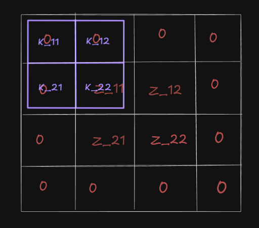
The difference in previous case and this one, is that the sizes of both operand matrices were in our favour. Here even if we try to brute force the same thing, we cannot hope to achieve any desirable results because the size of both, kernel and error signal matrices is same which is 2 × 2.

So we apply padding of 1 on the error signal matrix, which makes it 4 × 4, and (4-2+1) is 3, so we will get a 3 × 3 matrix. This is good. But there’s still a catch.

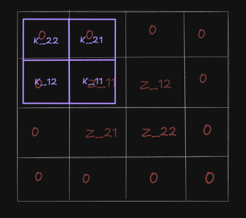
From this image you can see, that while trying to attempt the convolution, we are getting false result for the very first equation. We need Z_11 to match with K_11 to work. How can we achieve that? How about we rotate the filter matrix accordingly?

Now it looks better. You can try moving that filter over the rest of the matrix and you will obtain the exact same set of equations which we had.

To surmise what we did :

$$\frac{\partial L}{\partial X} = conv(\space padded(\frac{\partial L}{\partial Z}) , 180^{\circ} \space rotated \space (K) \space )$$

But wait. Why did this happen? We didn’t do any rotation for the filter gradient? Why do we need it for the input gradient? Well, there’s a simple answer.

Intuition

The difference arises from the roles of Kernel and Input matrices:

• Input (X): During backpropagation, the error signal must "spread back" to the input. This reversal in the direction of convolution requires the 180° rotation of K to ensure proper alignment.

• Filter/Kernel (K): The filter weights are learned by summing up contributions from the input regions corresponding to each error signal position. The spatial alignment between K and X remains consistent with the forward pass, so no rotation is necessary.

With this, we have finally completed our backward pass. Now it’s time to implement this. We won’t need the equation for updating the biases since we haven’t used any.

def backward(self, dL_dout):

        dL_dinput = np.zeros(self.input.shape)
        dL_dfilters = np.zeros(self.filters.shape)

        for region, i, j in self.iterate_regions(self.input):
            for f in range(self.num_filters):
                dL_dfilters[f] += dL_dout[i, j, f] * region  
                dL_dinput[i:i+self.filter_size, j:j+self.filter_size] += dL_dout[i, j, f] * self.filters[f]

        # Update the filters
        self.filters -= self.lr * dL_dfilters

        return dL_dinput

This is the block of code which we will be adding to our previous implementation of Convolutional Layer. So it will finally look like:

class ConvLayer:
    def __init__(self, num_filters, filter_size, lr=0.01):
        self.num_filters = num_filters
        self.filter_size = filter_size
        self.filters = np.random.randn(num_filters, filter_size, filter_size) / 9
        self.lr = lr

    def iterate_regions(self, image):
        h, w = image.shape
        for i in range(h - self.filter_size + 1):
            for j in range(w - self.filter_size + 1):
                region = image[i:(i + self.filter_size), j:(j + self.filter_size)]
                yield region, i, j

    def forward(self, input):
        self.input = input
        h, w = input.shape
        output = np.zeros((h - self.filter_size + 1, w - self.filter_size + 1, self.num_filters))

        for region, i, j in self.iterate_regions(input):
            output[i, j] = np.sum(region * self.filters, axis=(1, 2))

        return output

    def backward(self, dL_dout):

        dL_dinput = np.zeros(self.input.shape)
        dL_dfilters = np.zeros(self.filters.shape)

        for region, i, j in self.iterate_regions(self.input):
            for f in range(self.num_filters):
                dL_dfilters[f] += dL_dout[i, j, f] * region  
                dL_dinput[i:i+self.filter_size, j:j+self.filter_size] += dL_dout[i, j, f] * self.filters[f]

        # Update the filters
        self.filters -= self.lr * dL_dfilters

        return dL_dinput

The only change other than the implementing the equations is to include the learning rate for updating the filters.

Now all which remains is to combine all this and test it on a sample image.

References

If you liked this, or want a visual understanding don’t forget to check out these videos by Learn with Jay. It helped me a lot and this explanation is based on these videos.

• Backpropagation in CNN - 1

• Backpropagation in CNN - 2