How Relational Databases work under the hood

What is the problem with B-Tree?

You know i wanted to build a databases but first step was learn about other databases in market so i can know how they work under the hood so after long nights and days wastage i came to know that The underlying data structure used in PostgreSQL and almost every relational database for storing data and fast retrieval is B-tree. B-tree is a self-balancing search tree data structure that stores data in a sorted fashion and does all operations — Search, Insert, and Delete in O(logn) complexity where n is the number of nodes in the tree.

Imagine a weary database engineer named Alex, toiling away in a dimly lit server room, surrounded by the hum of machines and the faint smell of burnt coffee. Alex had spent years mastering relational databases like PostgreSQL, marveling at their elegance—how SQL engines translated queries into execution plans, how B-trees kept everything neatly indexed, and how the system hummed along with ACID guarantees. Under the hood, these databases relied on a complex symphony: the SQL engine parsed queries using a lexer and parser, built an abstract syntax tree, and handed it to the query optimizer to choose the best path—maybe a B-tree index scan or a full table sweep. Data was stored in fixed-size pages (say, 8KB in PostgreSQL), with B-trees indexing rows by key for fast lookups. But Alex noticed something troubling as the database grew: every write rippled through the B-tree, splitting nodes, rewriting pages, and thrashing the disk with random I/O. To ensure durability, PostgreSQL used an append-only Write-Ahead Log (WAL)—a sequential file where every change was recorded before touching the main data files. This WAL, synced to disk, let the system recover from crashes by replaying logs, but it didn’t solve the write amplification problem. The heap files stored the actual rows, while B-trees indexed them, and a buffer manager juggled pages in memory. Triggers, constraints, and transaction managers added more layers, ensuring consistency but slowing ingestion as data scaled. Alex dreamed of something faster—something that leaned harder into append-only mechanics, sidestepping the B-tree’s limitations. That’s when the LSM tree caught their eye, promising a new way forward.

B-trees are optimized for balanced reads and writes. However, as the data grows, the B-trees based data storage engines start becoming a bottleneck because of write amplification.

What is write amplification? Whenever any write happens in a B-tree, it can lead to updating multiple pages of a database which would involve a lot of random disk I/O. This is called write amplification. Thus, the B-Tree limits how fast the data can be ingested into a SQL database.

What can we do better here? Enters the solution: LSM tree

Hint: Append only Logs

What is an LSM tree?

LSM tree stands for Log-Structured Merge tree. It’s a data structure popularly used in databases and file systems. It is optimized for fast writes. The LSM trees are a popular data structure choice for implementation in NoSQL databases. For example: Cassandra, SyllaDB, RocksDB. Let’s dive deep into it to understand better.

An LSM tree consists of two key components: Memtable and SSTables.

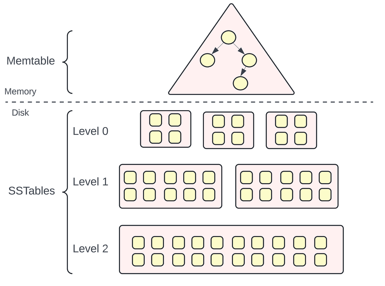
Memtable

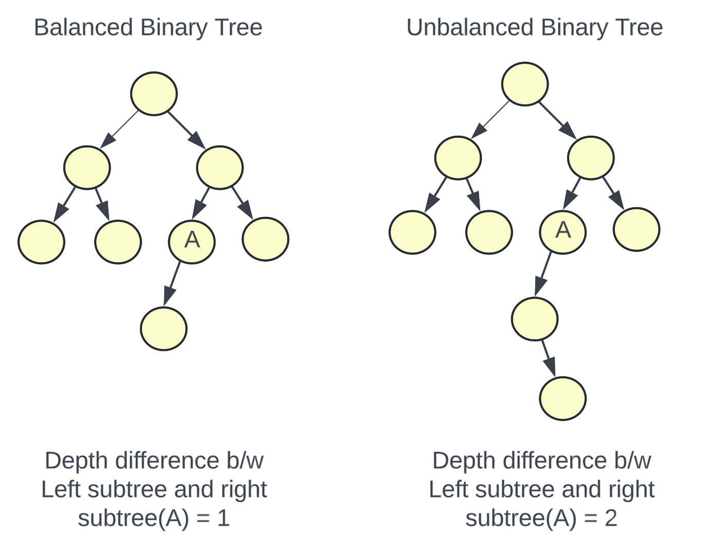
Memtable is a data structure that holds data in memory before it’s flushed into disk. It is usually implemented as a balanced binary search tree.

A balanced binary search tree is a data structure where the difference between the depth of the left subtree and the right subtree is 0 or 1 for every node. Since the tree is balanced, the height of a balanced binary tree is O(logN) where N is the number of nodes in the tree.

SSTables (Sorted String Tables)

SSTables stands for Sorted String tables. They contain a large number of <key, value> pairs sorted by the key. They are permanently persisted on the disk and are immutable i.e. the content in the SSTables cannot be modified.

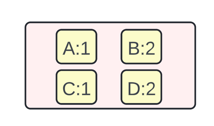
Representation of an SSTable containing <key, value> pairs

Compaction of SSTables

As more data comes into the database, more SSTables are created on the disk. The contents of SSTables are immutable to gain the advantage of Sequential I/O. Thus, if there is any update coming for the same key, it is also treated as a new write operation.

However, a large number of operations to the same key could lead to having multiple SSTables. If there are multiple SStables, the disk space usage might shoot up. To keep the disk space usage in check and avoid duplicate entries for the same key, there is a periodic compaction process of merging smaller SSTables into a larger SSTable. Once the merge is complete, the original Level 0 SSTables are deleted and no longer used.

So, you can imagine, that as more data comes into the database, the merge process kicks in when the space utilization reaches the configured threshold for a particular level. New SSTables are created at Level X + 1 and all the old SSTables at Level X are discarded.

For the following diagram, consider a few points:

Initially, all the <key, value> pairs in the SSTables at Level 0 are sorted by the key.
At Level 0, there are two operations for the Key:A. The first operation is Set(A, 1) and the second operation is Delete(A). When the compaction happens, the key:A is deleted and no longer present at the SSTable at Level 1.
There are two key, value pairs for the Key:C. The first one is C:1 and the second one is C:3. When the compaction happens, the latest key, value is taken into account for the same key and thus C:3 is retained in the new SSTable at Level 1.
You would realize now that merging SSTables is similar to the Merge algorithm of two sorted arrays.

There are different Compaction Strategies used in an LSM tree. For example: Size tiered compaction (optimized for write throughput) v/s Leveled compaction (optimized for read throughput). I’ll save this discussion for some other day.

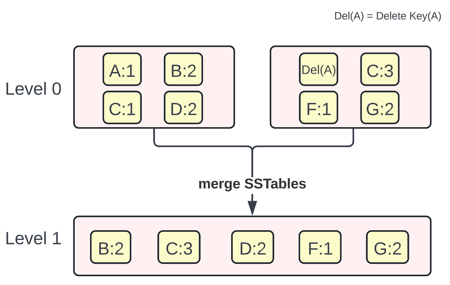
Representation of Compaction in LSM trees

Now that we’ve understood what are the key components of an LSM tree, let’s understand how Reads and Writes work in the case of a database that uses a Log-Structured Merge Tree.

How does a Write happen using an LSM tree?

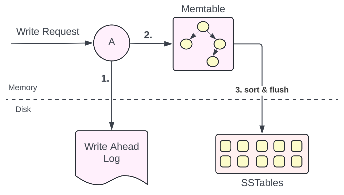
Representation of how a write occurs in a storage engine using an LSM tree.

When a write request comes to a database that uses an LSM tree, the write request change log is captured in a Write-Ahead Log file for durability. Read more about the Write-Ahead Log here.
Parallelly, the write request changes are stored in an in-memory structure called Memtable. As discussed earlier, memtable is usually implemented as a balanced binary search tree.
When the memtable reaches a certain threshold, the memtable is sorted and all the data is flushed to the disk in the form of SSTables (Sorted String tables).

How does a Read happen using an LSM tree?

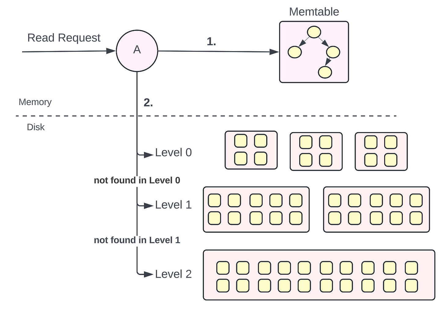
Representation of how a read occurs in a storage engine using an LSM tree.

When a read request comes, the key is first searched in the in-memory memtables. If the key is found, the value is returned at lightning-fast speed because of faster access from memory compared to the disk.
If the key is not found in the memtables, it is searched on the disk. Firstly, it is searched on the Level 0 SSTables, then the Level 1 SSTables, then the Level 2 SSTables, and so on.

Optimization on Reads

Since the SSTables are sorted in nature, we can do a logarithmic search to find the desired key. Still, the logarithmic search would be a costly read because we would be doing a lot of disk I/O operations to figure out if a key exists in the SSTables at a particular level or not.

What can we do better to optimize the reads further? Remember Bloom filters?

Bloom filters are a space-efficient probabilistic data structure that helps in solving the problem: “Does the element exist in the set (data structure) or not?”

We can implement a bloom filter data structure per Level of the LSM tree to represent if a particular key exists in the Memtable/SSTables at a particular level or not. We know that there could be some false positives but we would end up scanning the whole Level much faster compared to doing a Logarithmic search on all the SSTables at every level. Memtable is also not an exception here. Checking if the key exists in bloom filters would be much faster on average compared to reading the self-balancing tree of the memtable in memory.

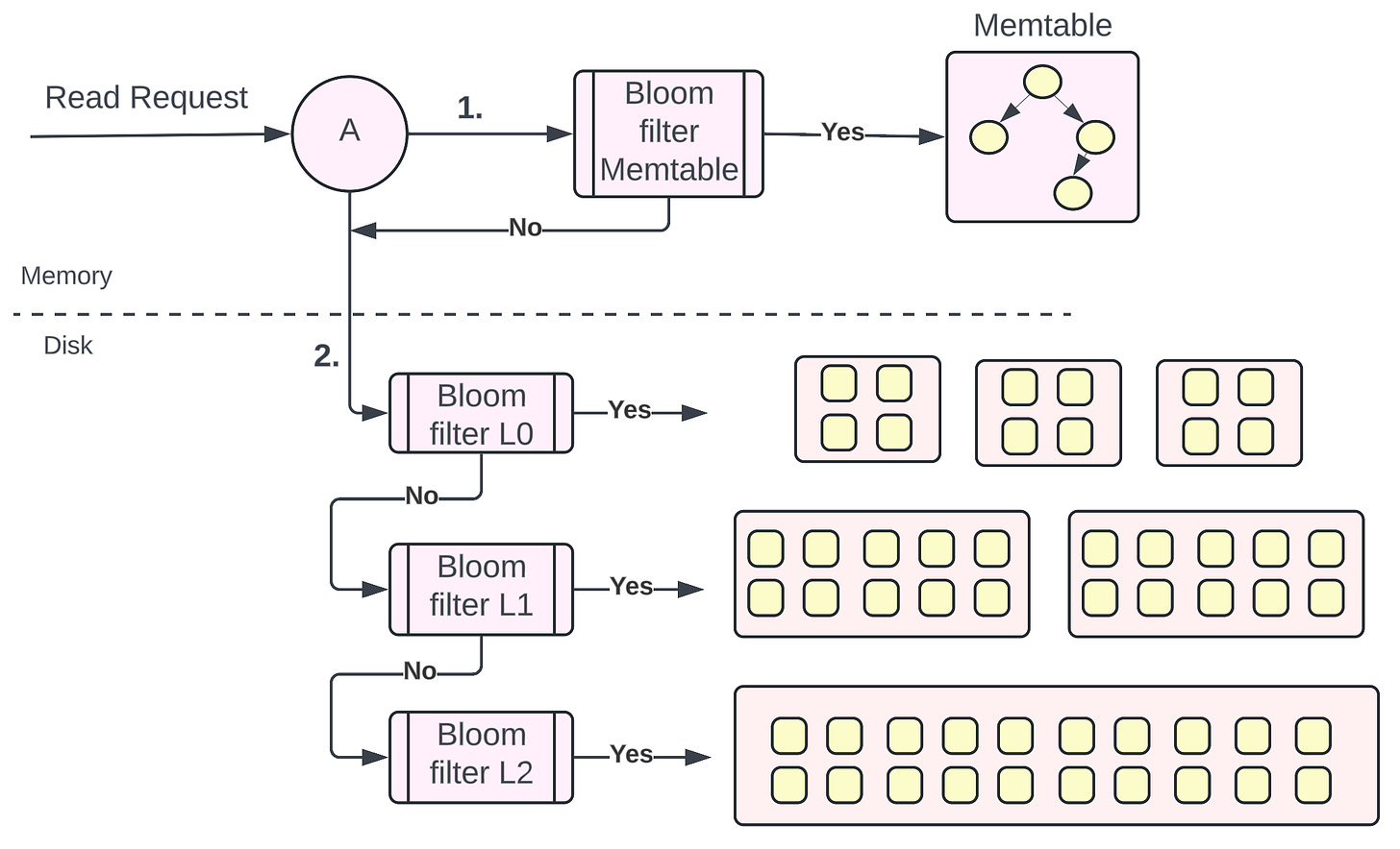
Representation of how bloom filters can speed up reads

Conclusion

Well, that’s about LSM trees. What’s important to realize here is how LSM trees are so efficient for heavy write throughput due to the append-only nature of the SSTables. This is because of Sequential I/O — the same factor when we discussed about why Kafka is fast.

It’s also important to understand writing to a WAL is also the same approach used in PostgreSQL but the underlying data structure (B-tree used in PostgreSQL) is different from the LSM trees used in Cassandra.

Also, LSM trees find their application in various real-world systems: NoSQL databases, Search Engines, Time-Series databases, etc. I will mention more about this in the future when case studies are discussed.

I hope this discussion is worth it for your future needs. That’s it, folks for this edition of the newsletter.

How Relational Databases use under the hood LSM Trees algorithm