Hi there! 👋

I’m Dhyuthidhar, and if you’re new here, welcome! I love exploring computer science topics, especially machine learning, and breaking them down into easy-to-understand concepts. Today, let’s discuss neural networks.

In the previous blog, I discussed several functions essential for developing logistic regression. Now, let’s delve into the mathematical foundation of neural network code, starting from the basics to making predictions.

Perhaps I’m diving straight into the deep learning series, skipping over parts of the ML series. However, if you’ve read my previous blog, this will be the perfect follow-up in that ML series for you to explore.

Previous blog: Link

So in this code, I will explain to you the neural network using the make_moon data in the sklearn.

• Let me tell you the characteristics of the data:

  • There are 400 examples in the data.

  • There are 2 features in the data.

Importing the necessary libraries

# This notebook implements a neural network with one hidden layer for binary classification
# on the make_moons dataset from scikit-learn.

import numpy as np
import matplotlib.pyplot as plt
from sklearn.datasets import make_moons
import copy

# Set random seed for reproducibility
np.random.seed(3)

• I explained to you all these modules in the last blog, and I will give you a summary here:

  • We utilize NumPy for mathematical computations, Matplotlib for data visualizations, scikit-learn (sklearn) for machine learning models and operations, and the copy module to duplicate variable data.

• Set a random seed to ensure the results of this code are reproducible.

Importing the data

# Generate a moon dataset using sklearn as a replacement for the planar dataset
# The scikit-learn make_moons() function specifically generates a dataset that has two interleaving half-moons. 
# Each class (0 or 1) forms one of these half-moon shapes.

X_data, Y_data = make_moons(n_samples=400, noise=0.2, random_state=42)
X = X_data.T  # Shape: (2, 400)
Y = Y_data.reshape(1, Y_data.shape[0])  # Shape: (1, 400)

There are two matrices X and Y.

X.shape → (2,400)

• 2 features and 400 training examples

Y.shape → (1,400)

• 1 feature (label) and 400 training examples

• There are two labels, either 0 or 1

• These labels are used to create a full moon shape, with one part utilizing one class and the other part utilizing a different class.

Visualizing the data

# Visualize the data:
# We're plotting the two features of each data point on a 2D graph
# Why? The feature values in X are coordinates that, when plotted, create a moon-shaped pattern.
plt.figure(figsize=(8, 6))
plt.scatter(X[0, :], X[1, :], c=Y.reshape(-1), cmap=plt.cm.Spectral)
plt.xlabel('Feature 1')
plt.ylabel('Feature 2')
plt.title('Moon Dataset')
plt.show()

• All observation points from feature 1 will be placed along the x-axis, while all observation points from feature 2 will be positioned along the y-axis.

• A moon will form on that plane.

Know the shape of data

# We are going to find out the shape of X and Y
shape_X = X.shape
shape_Y = Y.shape
m = shape_X[1]  # Number of training examples

print ('The shape of X is: ' + str(shape_X))
print ('The shape of Y is: ' + str(shape_Y))
print ('I have m = %d training examples!' % (m))

• This is going to print the shape of X which is (2,400).

• The below line will print shape of Y which is (1,400).

• ‘m‘ represents the number of training examples which is 400,

Define Sigmoid Function

def sigmoid(z):

    s = 1 / (1 + np.exp(-z))
    return s

We will create the sigmoid function, which we will utilize to implement one of the layers of the neural network.

Simplest Logistic Regression using sklearn

from sklearn.linear_model import LogisticRegression

# Train logistic regression
clf = LogisticRegression()
clf.fit(X.T, Y.reshape(-1)) # We need to send features as columns and data as rows that why we are using transpose and instead of 2D y should be 1D so I am doing reshape to convert to 1D
# The sckitlearn Logistic Model expects the data in that way, so we need to convert them in that way before we fit data into the model.

• We are implementing a logistic regression model using the sklearn module, which handles all the mathematical computations in the background.

• Fit the data into that model.

• We transpose the X data and reshape the Y data to align with Sklearn's requirement, where features are represented as columns and data as rows, unlike our imported format with data as columns and features as rows.

• We are reshaping Y to convert the labels into a 1D format, ensuring the Y array meets the required structure.

Plotting decision boundary of Logistic Regression

# Plot the decision boundary for logistic regression
def plot_decision_boundary(model, X, y):

    # Set min and max values for plotting
    x_min, x_max = X[0, :].min() - 1, X[0, :].max() + 1
    y_min, y_max = X[1, :].min() - 1, X[1, :].max() + 1
    h = 0.01
    # Generate a grid of points
    xx, yy = np.meshgrid(np.arange(x_min, x_max, h), np.arange(y_min, y_max, h))

    # Run model prediction on all points in the grid
    if isinstance(model, LogisticRegression):
        Z = model.predict(np.c_[xx.ravel(), yy.ravel()])
    else:
        Z = model(np.c_[xx.ravel(), yy.ravel()].T)
    Z = Z.reshape(xx.shape)

    # Plot the contour and training examples
    plt.figure(figsize=(10, 8))
    plt.contourf(xx, yy, Z, cmap=plt.cm.Spectral, alpha=0.8)
    plt.scatter(X[0, :], X[1, :], c=y.reshape(-1), cmap=plt.cm.Spectral, edgecolors='k')
    plt.xlabel("Feature 1")
    plt.ylabel("Feature 2")
    plt.title("Decision Boundary")
    plt.show()

# Plot decision boundary for logistic regression
plot_decision_boundary(clf, X, Y)

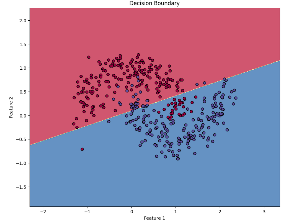
• This code extracts the minimum and maximum values of feature 1 and feature 2, then plots them on the x-y axis.

• The background colors show the decision boundary (where the model switches from predicting class 0 to class 1)

• You can see how the decision boundary separates two classes.

  

Calculate the accuracy of Logistic Regression

# Calculate accuracy for logistic regression
LR_predictions = clf.predict(X.T)
accuracy = 100 * np.mean(LR_predictions == Y.reshape(-1))
print('Accuracy of logistic regression: {:0.2f}%'.format(accuracy))
print("(percentage of correctly labelled datapoints)\n")

• We are taking the mean of the boolean array.

• The boolean array is created by checking whether the predicted values are equal to true values, and it generates a boolean array like [True, True, False, True].

• Python will convert that into [1, 1, 0, 1], where 1 is for true and 0 is for false.

• It calculates the mean and multiplies it by 100 to obtain the accuracy percentage.

Now let’s start to build the neural network model.

If you want to learn neural networks theoretically, you can check out my previous blog😉

Here it is: https://sudheendra.hashnode.dev/neural-networks-basics-vector-functions-and-math-behind-ai

Define the Layer sizes

def layer_sizes(X, Y):

    n_x = X.shape[0]  # Size of input layer
    n_h = 4           # Size of hidden layer (fixed to 4 for this exercise)
    n_y = Y.shape[0]  # Size of output layer

    return (n_x, n_h, n_y)

# Example usage of layer_sizes
(n_x, n_h, n_y) = layer_sizes(X, Y)
print("The size of the input layer is: n_x = " + str(n_x))
print("The size of the hidden layer is: n_h = " + str(n_h))
print("The size of the output layer is: n_y = " + str(n_y))

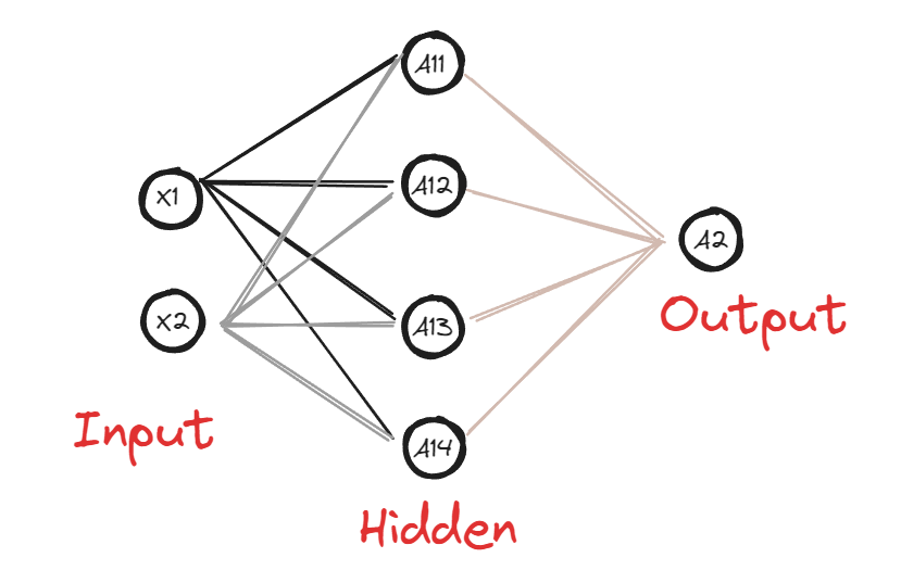
• The value n_x represents the shape of the input data, often referred to as the input layer. However, it is not considered an actual layer since it does not contain any neurons.

• The variable n_h defines the structure of the hidden layer, indicating the number of neurons it contains.

• The variable n_y defines the structure of the output layer, specifying the number of neurons present in it.

• We will initialize all these values in the layer_sizes function.

• The model performance depends on the number of neurons in the hidden layer; if there is no hidden layer, it will look similar to the logistic regression, so the hidden layer plays an important role.

• You can play with the shape of the hidden layer and see how it affects the output of the model.

  

Initialize the parameters

def initialize_parameters(n_x, n_h, n_y):

    # Backpropagation and gradient descent can only work well if they have a good starting point.

    np.random.seed(2)  # For consistent initialization

    # Initialize weights with small random values to break symmetry
    W1 = np.random.randn(n_h, n_x) * 0.01 # So that gradients that are generated wont be too small or too large
    b1 = np.zeros((n_h, 1))
    W2 = np.random.randn(n_y, n_h) * 0.01
    b2 = np.zeros((n_y, 1))

    parameters = {"W1": W1,
                  "b1": b1,
                  "W2": W2,
                  "b2": b2}

    return parameters

# Example usage of initialize_parameters
parameters = initialize_parameters(n_x, n_h, n_y)
print("W1 = " + str(parameters["W1"]))
print("b1 = " + str(parameters["b1"]))
print("W2 = " + str(parameters["W2"]))
print("b2 = " + str(parameters["b2"]))

• We use np.random.seed(2) to ensure that the random values generated remain consistent every time the code is executed. The number 2 is arbitrary and can be replaced with any value. Without this initialization, the values for w1 and w2 would differ each time the code runs.

• We will initialize the weights with two values corresponding to the input size of 2, along with two values for the bias. Finally, we will return the parameters.

• So now you can have a question like:

  • Why are we multiplying using 0.01 for weight initialization? Weight initialization plays a crucial role in deep learning. If the weights are initialized too small, it can lead to insufficient signal propagation through the network*, causing the model to learn very slowly. On the other hand, initializing weights with excessively large values may lead to* vanishing gradients (for sigmoid/tanh) or potential exploding gradients (especially in deeper networks). To address this, we use a multiplier of 0.01 for weight initialization, as it strikes an optimal balance.

  • Why do we emphasize proper weight initialization at the beginning, even though backpropagation adjusts them later? We do this because if the initialization of weights does not work well, there is a risk that gradient descent may lead to vanishing or exploding gradients, or become trapped in poor local minima. As a result, the optimization process (backpropagation) fails before it can function effectively.

  • Why did we initialize weights to 0 in the logistic model but not in this case? In logistic regression, weights are typically initialized to 0 without any issues. However, doing the same in a neural network leads to the symmetry problem. This issue arises because all neurons in a given layer compute the same output, resulting in identical gradients during backpropagation. Consequently, the neurons remain indistinguishable throughout training. Additionally, while logistic regression deals with a convex function (which has a single global minimum), neural networks involve non-convex functions that contain multiple local minima. This makes it challenging for gradient descent to converge to the global minimum.

Forward Propagation

def forward_propagation(X, parameters):

    # Retrieve parameters from the dictionary
    W1 = parameters["W1"]
    b1 = parameters["b1"]
    W2 = parameters["W2"]
    b2 = parameters["b2"]

    # Implement Forward Propagation to calculate A2
    Z1 = np.dot(W1, X) + b1
    A1 = np.tanh(Z1)
    Z2 = np.dot(W2, A1) + b2
    A2 = sigmoid(Z2)

    assert(A2.shape == (1, X.shape[1]))

    cache = {"Z1": Z1,
             "A1": A1,
             "Z2": Z2,
             "A2": A2}

    return A2, cache

# Example usage of forward_propagation
A2, cache = forward_propagation(X, parameters)
print("A2 = " + str(A2))

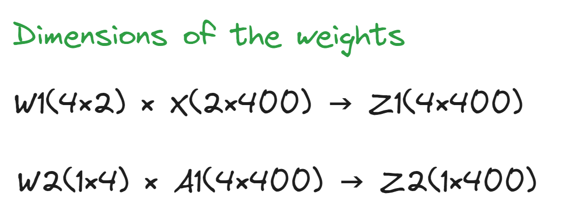
• We are going to take X and parameters as the argument for the forward_propagation function.

• We will implement the Z1 and Z2. The formulas are as follows:

$$Z i ​ =W i ​ ⋅X i ​ +b i$$

• We proceed to implement A1 and A2. In A1, the tanh function serves as the activation function for the hidden layer, while in A2, the sigmoid function is utilized as the activation function for the output layer.

• Why do we use two different activation functions for two different layers? We use the sigmoid function in the output layer because we are performing binary classification. For the hidden layer, we opt for the tanh activation function for three key reasons:

  • Zero-Centered Property: The tanh function has a zero-centered property, meaning its outputs are centered around zero. This helps the data to be distributed more symmetrically around this point.

  • Stronger Gradient Values: The maximum gradient value of tanh is 1, compared to sigmoid's maximum of 0.25. This stronger gradient helps mitigate the vanishing gradient problem during backpropagation.

  • Wider Range: Tanh outputs values in the range (-1, 1), whereas sigmoid outputs values in the range (0, 1). The wider range of tanh provides neurons with greater representational power.

Conclusion

In this first part of our neural network exploration, we've covered the foundational elements of building a neural network with one hidden layer from scratch. We've seen how this architecture can effectively solve problems that simple logistic regression cannot, particularly with non-linearly separable data like our moon-shaped dataset.

Key takeaways from this implementation include:

1. Data Structure Matters: We've learned the importance of how data is organized (features as rows vs. columns) and how to transform between different formats.

2. Initialization is Critical: Random weight initialization is crucial for breaking symmetry in neural networks, allowing different neurons to learn different features. The scaling factor (0.01) helps maintain gradient flow during training.

3. Activation Functions: The use of tanh in hidden layers provides stronger gradients and zero-centered outputs, while sigmoid in the output layer gives us probability interpretations for binary classification.

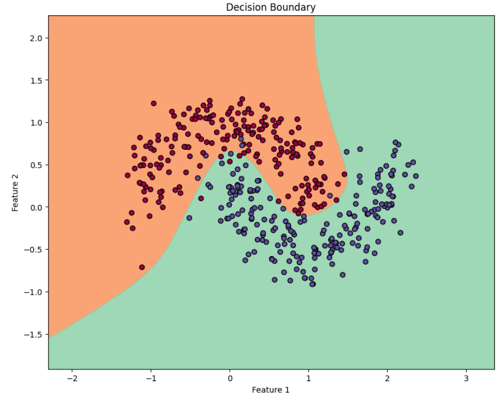
4. Beyond Linear Boundaries: Unlike logistic regression which can only create linear decision boundaries, neural networks with even just one hidden layer can create complex, non-linear decision boundaries.

5. Forward Propagation: We implemented the forward pass that transforms inputs through weighted connections and activation functions to generate predictions.

In the next part, we'll explore the forward propagation and backward propagation process to understand how the network learns from its mistakes and complete our implementation with the training and evaluation processes.

This hands-on approach to understanding neural networks provides much deeper insights than simply using pre-built libraries, giving you the foundational knowledge to tackle more complex architectures in the future.

References

These are the references that will be helpful to get to know more about this concept:

1. Here is the code: One-Hidden-Layer Code

2. Deep Learning or Machine Learning course by Andrew Ng in Coursera (Week 3 in course 1).

3. The 100 Pages of ML book by Andriy Burkov

4. Logistic Regression Code Introduction Part-1 blog

These two are wonderful resources for learning these concepts.

Action Step:

Let's create a tiny dataset with just 3 examples, 2 features, and binary labels:

X (2×3 matrix, features as rows):

X = [
    [1.0, 0.5, -0.5],  # Feature 1
    [0.3, 1.0, -0.1]   # Feature 2
]

Y (1×3 matrix, labels):

Y = [[1, 0, 0]]

Here’s a simple dataset for you to work with. Try implementing a neural network model using this data.

You can also practice the concept by working it out on paper.

Why I Share This

Simon Squibb believes that the best way to share knowledge is to make it simple and accessible. That’s exactly what I do—I break down complex technology into something easy and exciting.

Tech should inspire you, not intimidate you.

Imagine a world without machine learning—every company would need to manually analyze massive datasets just to extract insights. Deep learning changed that game. It enables anyone with data to uncover patterns and build intelligent systems without relying solely on traditional methods.

I share knowledge this way because I want you to feel that excitement too.

If this post made you think differently about tech, check out my other blogs. Let’s make tech easy and exciting—together! 🚀