Heavy Map Visualizations Fundamentals for Web Developers
 Advena
Table of contents
So, you’ve reached a point where your web application needs to display a map—not just a simple one with a single marker, but one that overlays a large dataset. Maybe the data points move, update in real time, or need to be interactive.
If you’ve worked with maps in web applications before, you might have only embedded a Google Map to show a restaurant’s location. Now, you’re working on something much more complex. How can you display a huge number of data points without your application slowing down? How do you keep animations and interactions smooth?
This guide introduces you to the basics of showing large datasets on maps. We will cover essential ideas, explain key terms, and give you an overview of the techniques that keep your app fast and responsive.
Note
This guide is about displaying the large datasets for maps, not about how to create or manage it. Making these specific datasets is a different discipline often handled by data specialists, or engineers using AI-driven analysis. Usually, the data you use will come from an internal data team, an external provider, or an open dataset that you want to show on your service.
Our goal is to help you take that data—no matter where it comes from—and present it in an efficient, interactive, and user-friendly way.
Before we begin, let’s define the type of data you’ll be using: Geospatial Data.
1. What Is Geospatial Data?
Geospatial data is any information that is tied to a specific location on Earth. It goes beyond just placing a marker on a map—it allows you to analyze and interact with data based on location.
For example, a simple map might drop a pin at a restaurant using coordinates or an address. However, geospatial data gives you more capabilities, such as:
Finding nearby places: Determine what’s close to a user’s current location.
Tracking movement: Monitor delivery routes or user activities over time.
Creating heatmaps: Visualize areas of high or low activity.
Setting up geofences: Trigger actions when someone enters or leaves a specific area.
To represent this data on maps, we use simple geometric shapes called vector shapes. If you’ve ever worked with SVGs or HTML Canvas, these concepts should be familiar. In geospatial applications, there are three main types of vector shapes:
Points: Represent a single location (like a restaurant or landmark) using latitude and longitude.
Polylines: Connect multiple points creating lines to illustrate roads, paths, or routes (Poly-lines are simply multiple connected lines).
Polygons: Form closed shapes to represent areas such as city boundaries, parks, or regions.
Websites like Ventusky use geospatial data to display live weather patterns, wind speeds, and temperatures across the globe. Similarly, FlightRadar24 shows real-time air traffic on maps.
Example: A Ferry Route in New York
Imagine a ferry traveling between two points:
Start Point: Near the Statue of Liberty.
End Point: At South Ferry Port.
Now, assume there is a restricted military zone on the water. You could draw the ferry’s path manually, but with geospatial data, you can also create a safe route automatically by avoiding the restricted zone.
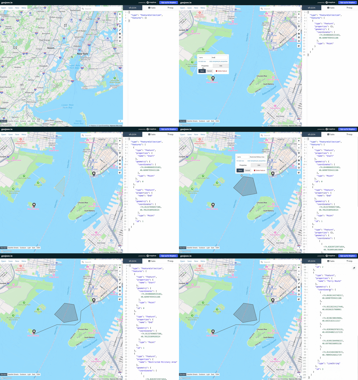
In summary, geospatial data includes any location-based information, and using vector shapes such as points, polylines, and polygons helps turn that information into maps that support analysis and decision-making.
Tip: If the term “geospatial data” ever feels overwhelming, just think of them as vector shapes with geographic information tied to them.
What About GIS?
When working with geospatial data, you might also hear about Geographic Information Systems (GIS). A GIS is an application that helps collect, store, analyze, and display geospatial data. Think of geospatial data as the raw information and GIS as the tool that makes sense of it. One popular GIS application is QGIS, which is free and open source.
2. Fundamentals of a Geospatial App
Let’s break down the key parts of a geospatial web app.
2.1 The Map Itself
Every geospatial app starts with a base map. The base map is the foundational background layer that shows essential details like roads, cities, water bodies, landmarks, and place names. It serves as the canvas on which you display your own data on. Building these base maps is a complex process that involves using large, detailed satellite images, or managing millions of geospatial data (vector shapes with geographic information) to represent the world.
The good news is that you do not need to create the base map from scratch. There are many existing services that offer ready-made base maps
OpenStreetMap (OSM) – A free and open-source base map.
Google Maps – We all know this one.
Mapbox – A popular alternative to Google Maps
Example: Creating a Base Map using Vector shapes
You can represent the world using geospatial data. This is done by people who draw vector shapes on top of satellite images images and label them with meaningful information.
The GIF below illustrates how vector data is created for an island: start by drawing the shape of the island, then label the island with the name "Dangar Island."
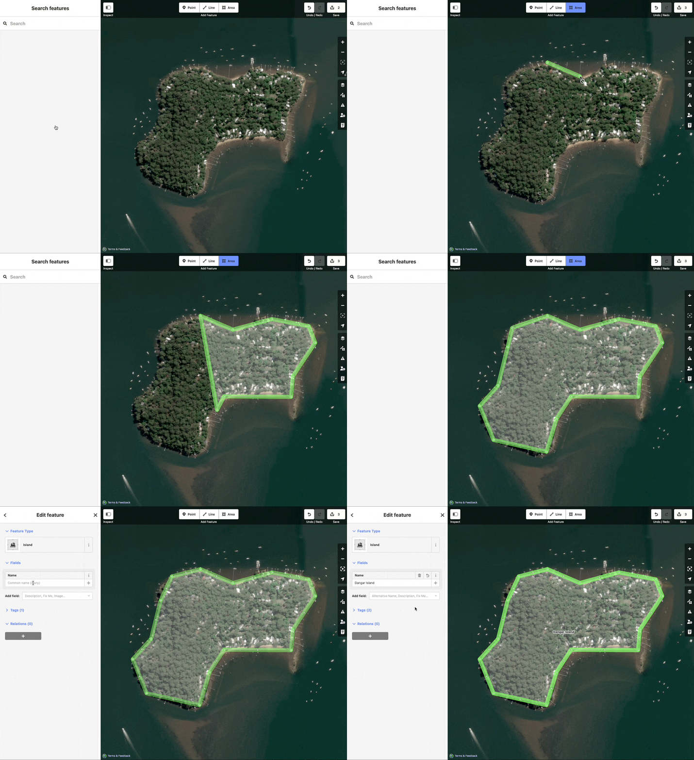
What you saw in the GIF is actually the creation of geospatial data: the island's shape is drawn with a polygon and it is labeled as an island with the name "Dangar Island".
Repeat this process for all roads, forests, cities, neighborhoods, and other features around the globe, you end up with a complete base map of the world.
2.2 Your Geospatial Data (What You Want to Display)
After you have chosen your base map, you can add your own geospatial data. This extra layer of information is what makes your application unique, whether you are displaying locations of restaurants, animal habitats, delivery routes, or anything else that benefits from a visual map.
One common format for storing geospatial data is in GeoJSON (files ending with .json or .geojson). GeoJSON is simply a JSON format that follows a specific structure for geospatial data. Here’s a simple example representing a bus station:
{
  "type": "FeatureCollection",
  "features": [
    {
      "type": "Feature",
      "geometry": {
        "type": "Point",
        // Coordinates are stored in [longitude, latitude] order
        "coordinates": [-73.983, 40.761]
      },
      "properties": {
        "station_id": "12345",
        "handicap_friendly": false
      }
    },
    ...
  ]
}
Other file formats you might see include:
Shapefiles (
.shp) – A legacy format used in many desktop GIS programs like QGIS. It is considered outdated for modern use.GeoPackage (
.gpkg) – A modern, efficient alternative for large datasets with better querying capabilities.
Although GeoJSON is straightforward to work with, geospatial data often involves thousands or even millions of points, which can create very large files. These files sometimes exceed 100 megabytes in size. Managing this data efficiently is key. In this guide, we will mostly work with GeoJSON for demonstration purposes because it's easy to read and work with, but it’s not the best for storing or serving large datasets.
As you advance in this guide, you will understand and explore more efficient data formats.
2.3 Data Source (Where Your Data Comes From)
There are many ways to store your geospatial data.
You can serve it as GeoJSON from your backend or store and deliver GeoJSON files using cloud storage services like AWS S3, Backblaze B2, or Google Cloud Storage.
For more complex needs, consider using a database like PostgreSQL or a specialized hosting service such as Mapbox.
Additionally, numerous public datasets provide free geospatial data, such as [NYC taxi trips], which are stored in Parquet—a popular alternative to the Shapefile format.
2.4 Putting everything together
Now that you have your base map, geospatial data, and a source for that data, it’s time to combine them!
You use JavaScript libraries to render your base map, request your data, and then handle and display the geospatial data using various vector shapes.
Many JavaScript libraries let you easily add markers, routes, and shapes to your map. Some libraries focus solely on rendering the base map, while others are designed to handle heavy data layouts. We will introduce these libraries later in the guide.
2.5 Quick Recap
Here are the main components of a geospatial web app:
Base Map: The background map that shows roads, landmarks, and cities. Examples include OpenStreetMap, Google Maps, or Mapbox.
Your geospatial Data: The custom data you want to display that makes your app unique.
Data Source: Where your data lives—this could be a database (e.g., PostgreSQL), your own backend, cloud storage (S3, Backblaze B2, GCS), or a public dataset.
Putting Everything Together: Use JavaScript libraries to overlay your data (markers, routes, shapes) on the base map.
3. Our First Map
Let's begin by selecting the JavaScript library to build interactive maps for your web applications.
Some JavaScript libraries are designed to work with any base map service (Google Maps, Mapbox, OpenStreetMap,...), while others restrict you to only one. This coupling can significantly affect costs and scalability over time, as services like the Google Maps API are known for their high expenses under heavy usage. Your early choice of a JavaScript library can therefore impact your project's cost structure and growth potential, making it essential to balance functionality, flexibility, and expense.
3.1 Popular JavaScript Map Libraries
You may have used one of these libraries before:
Google Maps JavaScript API – Offers rich data, including real-time traffic and business listings. However, because it is tied to Google’s base map service, heavy usage can become expensive.
Mapbox GL JS – A high-performance and highly customizable library with many interactive features. Mapbox itself is a base map service with many other features, and offers a generous free tier. It’s generally less expensive than Google’s offering.
Leaflet – Great for simple, interactive maps. It’s lightweight and easy to use, but it isn’t built for heavy data visualization.
OpenLayers – A powerful and open-source option suited for professional GIS applications, though it has a steeper learning curve.
MapLibre GL JS – An open-source alternative to Mapbox GL JS that provides similar high-performance rendering without licensing issues.
The cool thing about Leaflet, OpenLayers, and MapLibre is that they are service-agnostic, meaning they can work with nearly any base map service.
3.2 Which One Should You Choose?
Our recommendation is to use MapLibre:
Developer-Friendliness: – MapLibre is regarded as very developer-friendly library. Unlike Leaflet, which is great for simple maps but lacks advanced features for heavy visualizations, MapLibre offers a richer set of tools that can handle complex projects more efficiently. OpenLayers might provide the same features, but is difficult to work with.
Ecosystem for Heavy Visualization: – MapLibre has a whole ecosystem built around it specifically designed for heavy visualization needs—a significant advantage over Leaflet and even OpenLayers, which do not offer as extensive support.
Flexibility: – Being open source and service-agnostic, MapLibre allows you to switch between base map providers, providing a sustainable solution for growing projects. This contrasts with Google Maps JavaScript API and Mapbox GL JS, both of which tie you to a particular service, potentially limiting your options and increasing long-term costs.
Is a fork of Mapbox GL JS – MapLibre is an open-source fork of Mapbox GL JS that began when Mapbox moved toward a more commercial business model. This means MapLibre retains many of the high-performance and customizable features that made Mapbox GL JS popular, without the same licensing or cost restrictions.
By choosing MapLibre, you gain the benefits of a developer-friendly tool that offers a robust ecosystem, unmatched flexibility, and cost-effective scalability—making it the best overall choice for your heavy mapping needs.
3.3 Let's Build a Map with Markers
In this guide, we’ll write our code in React which probably is the most popular library for building single-page applications. Much of this code can also be adapted for other frameworks.
Step 1: Installing the Dependencies
MapLibre is a pure JavaScript library, but there is also a React implementation, namely @vis.gl/react-maplibre.
Assuming you already have React set up, install MapLibre and its React components:
npm install --save @vis.gl/react-maplibre maplibre-gl
About Vis.GL
Vis.GL is an organization started by Uber. They develop libraries for complex geospatial applications. All of their libraries are open source, so you can expect reliable and high-quality tools for geospatial projects.
Step 2: Building the Map
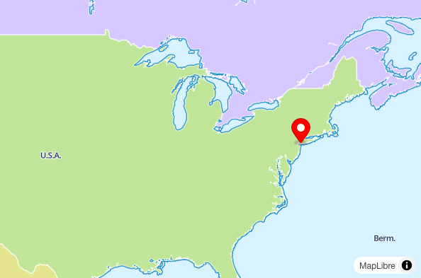
Here is some simple code that creates a map with a marker in New York:
import { Map, Marker } from "@vis.gl/react-maplibre";
import "maplibre-gl/dist/maplibre-gl.css"; // Required!

export default function App() {
  return (
    <Map
      initialViewState={{
        longitude: -80,
        latitude: 40,
        zoom: 3.5,
      }}
      style={{ width: 600, height: 400 }}
      mapStyle="https://demotiles.maplibre.org/style.json"
    >
      <Marker longitude={-73.924263} latitude={40.684388} color="red" />
    </Map>
  );
}
Pretty self-explanatory if you ask me: it creates a map that you can navigate, centered at a given latitude and longitude and places a red marker on it.
Later in this guide, we will look at example that uses external data sources like GeoJSON.
Did you notice that the map above is drawn using vector shapes, aka geospatial data? Notice that the United States (U.S.A) has a label, and it has a different color compared to Canada. The coastal areas are shown in dark blue, while the ocean is shown in a lighter blue.
4. Geospatial Data Formats
Up to now, we’ve talked about geospatial data as if it were always vector shapes—points, lines, and polygons with geographic information attached to them. While that’s true for many web applications tasks, geospatial data actually appears in two additional formats:
Raster – Think images or photos, like satellite views.
Tabular – Rows and columns (like CSVs), where each row has a location (coordinates or an address).
This distinction matters because geospatial data has existed for decades, originally created for specialized Geographic Information Systems (GIS) software. When you work on a modern web application, you will still encounter these formats for certain use cases.
Therefore, we can divide geospatial formats into three main categories:
Vector – The shape-based data you’ve seen already (points, lines, polygons).
Raster – Pixel-based images with geographic coordinates (like satellite photos).
Tabular – Spreadsheet-like files that list location details in rows.
Let’s explore each category in more detail.
4.1 Vector Formats
Let’s start with vector data, since you have already seen how web maps often use points, polylines, and polygons. Vector data is the most common in web maps because each item (for example, a point or polygon) can be styled or interacted with on its own.
Common vector formats include:
Shapefile (
.shp): Shapefiles are one of the oldest and most widely used formats in GIS. However, they’re not a single file—they come as a group (e.g.,.shp,.dbf,.shx, etc.) that work together. They have limitations such as a 2GB file size cap, restrictions on attribute name lengths, and limited support for complex geometries. While most desktop GIS software supports shapefiles, they are considered legacy in modern web applications.GeoJSON (
.json/.geojson): Basically a JSON that stores geographic data. Its JSON-based nature makes it easy to read and work with in JavaScript. However, it's very slow for large datasets - loading a 100MB GeoJSON file can take 10-20 seconds in a browser, while the same data in other formats might load in 1-2 seconds. Furthermore, to update even a small part of a GeoJSON file, you typically need to read the entire file, make your changes, and save it all again, not optimal when working with large datasets.FlatGeobuf (
.fgb): FlatGeobuf is a modern binary format optimized for fast reading and efficient storage. It is often 10–20 times faster than GeoJSON when dealing with large datasets. The trade-off is that, like GeoJSON, any update requires rewriting the entire file, so it’s best for static or rarely changed data.GeoPackage (
.gpkg): GeoPackage is a modern, open standard that stores geospatial data in a single binary file based on an SQLite database. It strikes a good balance between performance and flexibility. Unlike FlatGeobuf, GeoPackage allows you to update portions of the data without rewriting the entire file, making it ideal for projects where the dataset may change over time.
4.2 Raster Formats
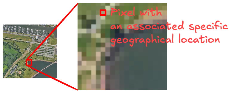
Raster formats represent maps as grids of cells (similar to pixels). Think of a satellite photo where each pixel contains information about the area it covers (like elevation or land cover). Common raster formats include GeoTIFF, JPEG (with georeferencing), and PNG (with georeferencing).
4.3 Tabular Formats
Sometimes you'll deal with geospatial data comes in tabular form, like CSV or Excel spreadsheets. These files list locations (with longitude and latitude) and additional data (like names or populations). They don’t usually store shapes or areas, but it's common to include GeoJSON strings in columns as a workaround.
4.5 Choosing the Right File Format
When deciding which geospatial file format to use, it helps to think about the size of your data, how frequently it changes, and how fast you need to load it in your web application.
Geospatial data can be quite large, often several 100MB in size.
For many projects, GeoJSON is appealing because it’s just JSON—a format that is familiar, human-readable, and easy to parse in JavaScript. However, while GeoJSON is great for smaller datasets and quick prototypes, it can become inefficient with larger datasets. Its text-based nature can lead to slow parsing when datasets become very large, and updating even a small portion typically means rewriting the entire file.
If you have a bigger, more complex dataset that must load quickly for end users, you might consider FlatGeobuf. Its binary format often delivers faster performance than GeoJSON, especially for large datasets. The main drawback is that any update still requires recreating the file, making FlatGeobuf best suited for information that doesn’t change frequently.
For projects that need to update data more often, or that require multiple layers in a single container, GeoPackage might be a better fit. It’s built on a lightweight SQL database, which means you can edit just the parts of the dataset that need changing. You also get the convenience of having everything in a single file.
Whichever format you pick, it’s worth remembering that in many workflows, these files are just a temporary way of sharing or transporting data. You might choose to import them into a database once you receive them, or convert them into something else for optimized web performance.
In other words, these formats aren’t always used directly in the browser; sometimes they’re just intermediate steps between a data provider and your live web application. The right choice depends on your project’s needs, but we will discuss that more soon.
In summary:
GeoJSON is easy to work with for small projects, but it becomes slow as datasets grow.
FlatGeobuf is much faster than GeoJSON for large, static datasets where you just need to store and quickly load the data
GeoPackage offers a good balance, allowing you to update parts of your dataset without rewriting the whole file—ideal if your data changes over time.
Often, these formats are just the first step. Once you receive the data, you might later import it into a database to optimize performance, flexibility and security.
You do not need to learn binary data formats to work with FlatGeobuf or GeoPackage. Usually, you will use libraries and tools that handle them for you.
Remember: For demonstration purposes, this guide relies heavily on GeoJSON because it’s extremely easy to read and parse in JavaScript. However, for larger or more dynamic projects, you’ll want to explore the other formats to find one that meets your performance and flexibility needs.
A more complete list of formats can be found here
4.6 Understanding the GeoJSON Structure
Looking at GeoJSON helps you understand what is usually stored in a geospatial data format.
From our memory aid—“geospatial data = vector shapes with geographic data”—GeoJSON is a way to store these shapes (points, lines, or polygons) along with additional data in a JSON file. In GeoJSON, each shape along with its related information (like a name or category) is known as a Feature.
At the highest level, a GeoJSON file is generally a FeatureCollection, which means it holds a list of features. Each Feature contains a geometry and a set of properties:
The geometry describes the shape type—“Point,” “LineString,” (for polyline) or “Polygon”—as well as the coordinates (longitude and latitude) that define where the shape is located.
The properties object is where you can store any additional data about that shape, such as a city’s name, a park’s opening hours, or a route’s ID.
Here is a simplified GeoJSON example showing a single Feature for a point location:
{
  "type": "FeatureCollection",
  "features": [
    {
      "type": "Feature",
      "geometry": {
        "type": "Point",
        "coordinates": [-74.006, 40.7128]
      },
      "properties": {
        "name": "New York City",
        "description": "Example of a point feature."
      }
    }
  ]
}
"type": "FeatureCollection" indicates this is a container holding one or more features.
"features" is the array that lists all the individual features.
Each item in this array has "type": "Feature", along with "geometry" (here it’s a
"Point") and "properties" ("name"and"description")."coordinates" is always written as
[longitude, latitude].
4.7 Preferred Order for Latitude & Longitude
In programming, coordinates are often stored as arrays (like [-87.73, 41.83]) instead of objects (like { lng: -87.73, lat: 41.83 }). This practice has led to different implementations over time, wreaking chaos due to mismatches in coordinate order. For example, one format places a point in Chicago, while another places it deep in Antarctica.
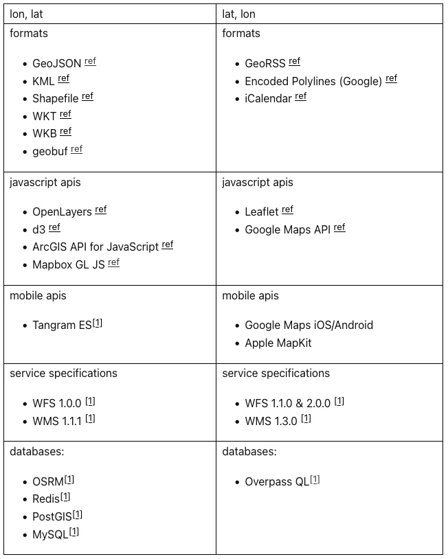
The table below shows which tools or file formats use which order for coordinates.
As a general rule of thumb, it's best to use longitude, latitude (lon, lat).

Source: MacWright.com
4.8 Example: Rendering GeoJSON
Imagine we have a GeoJSON file with thousands of features, hosted at https://example.com/largeData.json. A simple way to show these points on a map is to loop through each one and display it.
import { useEffect, useState } from "react";
import { Map, Marker } from "@vis.gl/react-maplibre";
import "maplibre-gl/dist/maplibre-gl.css"; // Required!

export default function App() {
  const [largeData, setLargeData] = useState<Record<string, number>[]>();

  useEffect(() => {
    fetch("https://example.com/largeData.json")
      .then((resp) => resp.json())
      .then((data) => setLargeData(data));
  }, []);

  return (
    <Map
    // ...
    >
      {largeData &&
        largeData.map(({ id, longitude, latitude }) => (
          <Marker
            key={id}
            longitude={longitude}
            latitude={latitude}
            color="red"
          />
        ))}
    </Map>
  );
}
This method might be fine for a small set of data. However, if you have tens of thousands of markers, each <Marker> is actually an <svg> element. In MapLibre and similar libraries, when you move or zoom the map, the browser must reposition each of these SVG elements using CSS transforms. Recalculating positions for each element is a massive overhead.
Instead, imagine we would render all data points in one layer and let the GPU (Graphics Processing Unit) handle the heavy lifting. Modern GPUs are designed to perform thousands of similar operations simultaneously.
This is where Deck.gl comes in.
5. Deck.gl
Deck.gl is a library from Vis.gl (the same team behind our MapLibre React wrapper) designed specifically for visualizing large geospatial datasets with WebGL. It works in any JavaScript environment—whether you use React, Vue, Angular, or vanilla JavaScript.
One of Deck.gl’s key features is its layer-based approach to rendering data. For example, here’s how you can use Deck.gl’s ScatterplotLayer, which simply creates a layer of marker points on a map, to visualize multiple locations:
import { useEffect, useState } from "react";
import { DeckProps } from "@deck.gl/core";
import { ScatterplotLayer } from "@deck.gl/layers";
import { MapboxOverlay } from "@deck.gl/mapbox";
import { Map, useControl } from "@vis.gl/react-maplibre";
import "maplibre-gl/dist/maplibre-gl.css";

// Wrapper to render DeckGL Layer on top of Maplibre
function DeckGLOverlay(props: DeckProps) {
  const overlay = useControl<MapboxOverlay>(() => new MapboxOverlay(props));
  overlay.setProps(props);
  return null;
}

interface Point {
  id: number;
  latitude: number;
  longitude: number;
}

export default function App() {
  // Create a layer to render many points using WebG
  const layer = new ScatterplotLayer<Point>({
    id: "ScatterplotLayer",
    data: "https://example.com/largeData.json",
    // Position expects [longitude, latitude] coordinates
    getPosition: (d) => [d.longitude, d.latitude],
    getFillColor: [255, 140, 0],
    radiusScale: 1000,
  });

  return (
    <Map
      initialViewState={{
        longitude: -80,
        latitude: 40,
        zoom: 3.5,
      }}
      style={{ width: 600, height: 400 }}
      mapStyle="https://demotiles.maplibre.org/style.json"
    >
      <DeckGLOverlay layers={[layer]} />
    </Map>
  );
}
Wit all markers placed on a single layer, Deck.gl can efficiently recalculate even 100.000 of them using WebGL behind the scenes.
5.1 Layers: The Building Blocks of Deck.gl
The key takeaway here is that in heavy web maps visualization, you want to work with layers. Deck.gl provides multiple types of layers to visualize different kinds of data. These layers serve as the foundation for rendering your geospatial data, with each one optimized for a specific type of visualization.
For example:
The
ScatterplotLayer(as seen in the example) is great for displaying points.The
HeatmapLayerhelps visualize the intensity of data points across a region.The
TripLayeris used for animated paths, such as tracking a taxi route from point A to B.
By combining different layers, you can create rich, interactive visualizations tailored to your data needs.
Deck.gl also makes it simple to load the data. Its data property can accept an array, an object, or even a URL pointing to a remote file. For example:
  const layer = new ScatterplotLayer<Point>({
    data: "https://example.com/largeData.json",
    // or
    data: [{ id: 1, latitude: 37.7749, longitude: -122.4194 }],
  });
Deck.gl natively supports JavaScript objects and .json files. If you need more formats, such as CSV or Geopackage, you can integrate loaders.gl. For example, to load data from a Comma-Separated Values (CSV) file:
  import {CSVLoader} from '@loaders.gl/csv';

  const layer = new ScatterplotLayer<Point>({
    data: "https://example.com/largeData.csv",
    loaders: [CSVLoader]
  });
This approach lets you fetch and parse many other file formats, allowing you to work with nearly any data source in your web maps.
5.2 What About Truly Huge Datasets?
When dealing with datasets containing millions of points or files exceeding hundreds of megabytes, even Deck.gl will struggle to render everything in a single layer.
While FlatGeobuf or Geopackage can significantly speed up data transfer to your web app, it does not improve Deck.gl’s rendering performance. Once the dataset is loaded, Deck.gl still needs to process and manage all the data. This means that while those other file formats reduces loading times, it won’t make rendering any faster.
To optimize performance, you can use techniques like simplifying geometries—for example, reducing the precision of latitude values from 40.9876543210 to 40.9876.
However, these methods have limits. When datasets become extremely large, a more scalable solution is required.
6. Tiling
When you are exploring web maps, you are likely to zoom and pan across huge areas, such as entire countries or even the entire Earth. As we mentioned earlier, the data for something like OpenStreetMap alone can reach over 100GB, and that is just for the street data—not counting imagery or other features. It would be impossible to download all of this data at once just to show a small corner of a city.
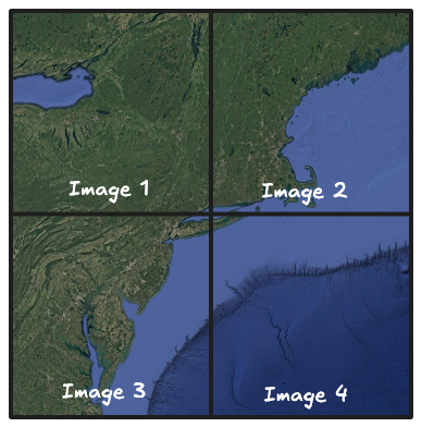
To solve this challenge, the mapping world relies on tiling. Tiling means we break the globe (or any large map) into smaller, more manageable squares called tiles. Each tile covers a specific geographic region at a particular zoom level. Rather than loading the whole map in one go, you only download the few tiles you need to display your current view. As you pan or zoom, new tiles are requested dynamically.
6.1 How Tiling Works
Tiles typically measure 256 by 256 pixels for raster images. You can imagine these tiles as puzzle pieces that fit together to form the map. But unlike a normal jigsaw puzzle, each piece is repeated multiple times at different zoom levels:
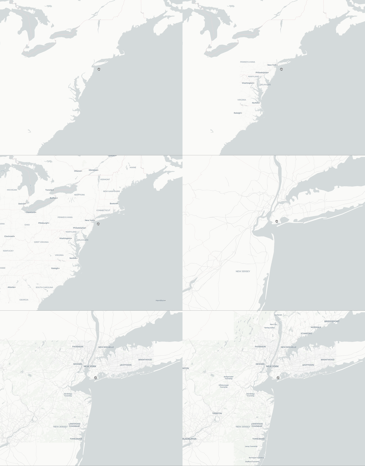
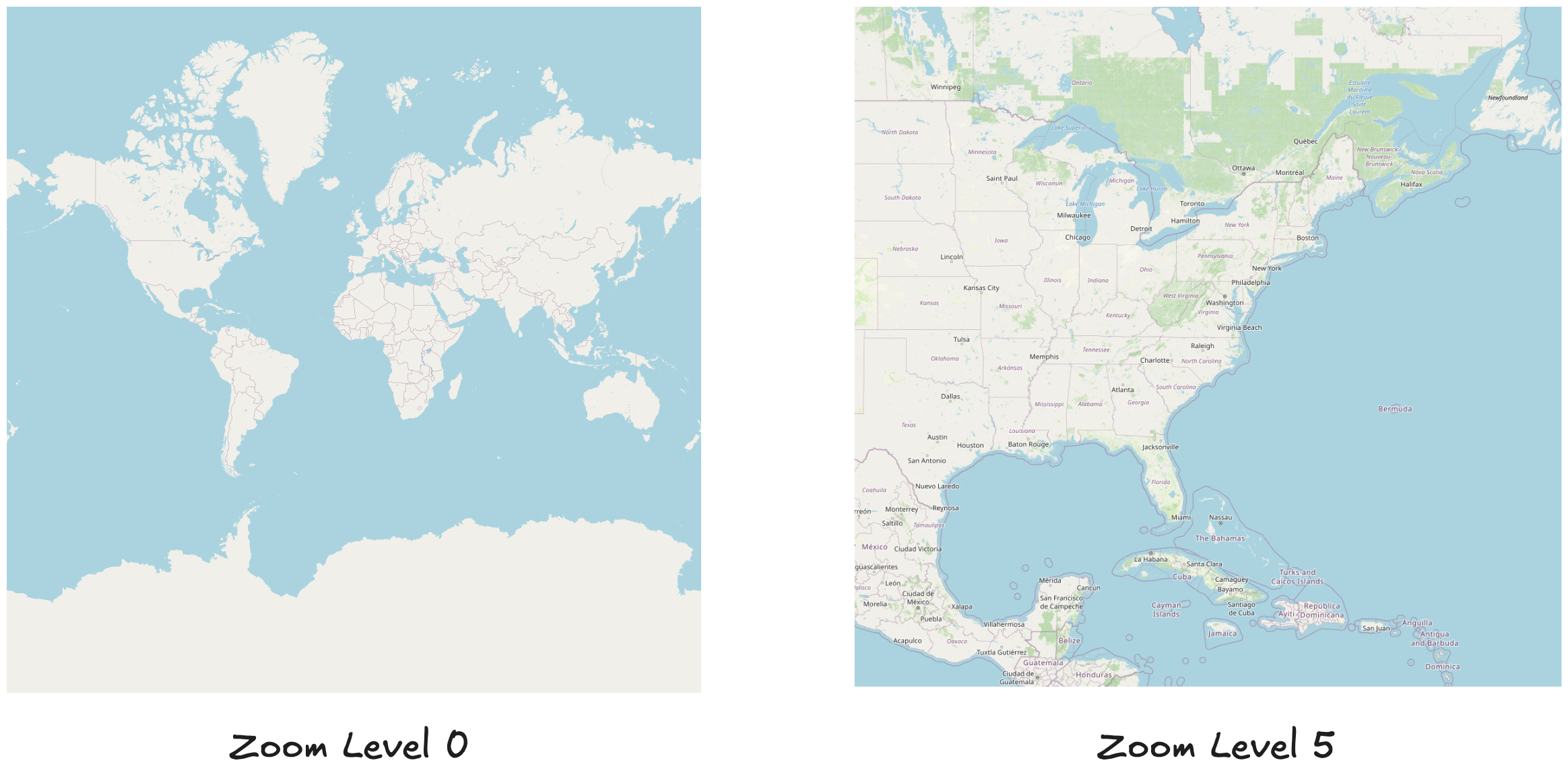
At lower zoom levels (e.g., zoom = 0 or 1, "zoomed out"): You see a very large region (like the entire world or a continent) within a small number of tiles. The data in those tiles is generalized or simplified to avoid clutter.
At higher zoom levels (e.g., zoom = 14, 15, "zoomed in"): The map shows more details for a smaller area. Each tile may contain a detailed slice of city blocks, roads, and buildings.
For example, the GIF below shows how zooming in on New York City brings in new, more detailed tiles:
Because each zoom level breaks the map into a grid, we identify each tile by a simple system known as XYZ coordinates:
Z is the zoom level,
X is the horizontal position of the tile,
Y is the vertical position of the tile.
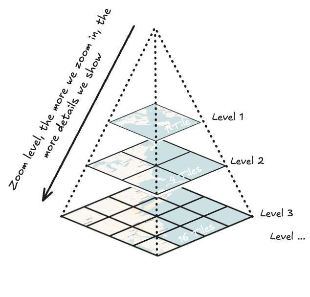
For example, at zoom level Z = 5, a tile might be identified as x = 9, y = 12. This corresponds to a particular rectangle on the map covering a certain region. If you zoom in to level 6, each tile at level 5 is replaced by four more detailed tiles at level 6.
Each zoom level increases the number of tiles exponentially.
| Zoom Level (Z) | Number of Tiles |
| 0 | 1 tile (covers the whole world) |
| 1 | 4 tiles (2 × 2 grid) |
| 2 | 16 tiles (4 × 4 grid) |
| 3 | 64 tiles (8 × 8 grid) |
| 4 | 256 tiles (16 × 16 grid) |
| … | … |
This means that every tile has a unique (X, Y, Z) value that identifies it.
6.2 Tile URL
A common URL pattern for requesting these tiles might look like:
https://my-tile-server.com/tiles/{z}/{x}/{y}.{format}
where .{format} could be a .png for raster tiles, or .pbf, which is a vector tile format that we will introduce shortly.
For example, if you are viewing New York City at zoom level 10, and the tile that covers Times Square has coordinates (X=302, Y=385), the URL to fetch that tile would be:
https://my-tile-server.com/10/302/385.png
Mapping libraries such as MapLibre or Leaflet automatically calculate which tiles to load as you interact with the map.
This URL method is called the XYZ Tile pattern (also known as the Slippy Map Tile scheme)—a system that was pioneered by Google.
6.3 Raster vs. Vector Tiles
Historically, tiles were raster images: small PNG or JPEG squares that stitch together seamlessly. If you have used earlier versions of Google Maps (back in 2005 or so), you have seen how these image tiles are loaded as you pan around.
Modern web maps are now built with vector tiles, which package the underlying geospatial data (roads, boundaries, and other geographic features) in a compact binary format. Because vector tiles send vector shapes than a flat image, your browser can render them. This leads to:
Smoother interaction: Moving and zooming around the map feels smoother
Less bandwidth usage: Sending tons of image files over the network can be inefficient, unlike simple binary data.
Easier visual styling: The map’s appearance (like roads, labels, building outlines) is defined in code (a style file). You can easily change colors, fonts, or line widths on the fly.
Raster tiles are still used for things like satellite imagery, because satellite photos are actual images and cannot be broken down into simple vector shapes. In practice, you might combine both: vector tiles for roads and boundaries, with optional raster tiles for aerial photography.
6.4 How MapLibre Uses Tiles Behind the Scenes
When you write code like this in React:
<Map
  initialViewState={{
    longitude: -80,
    latitude: 40,
    zoom: 3.5,
  }}
  style={{ width: 600, height: 400 }}
  mapStyle="https://demotiles.maplibre.org/style.json"
>
  {/* ...children */}
</Map>
You are passing in a mapStyle property, which is a URL to a style file in JSON format. This file defines how the map should look and where it should load tiles from. Inside this file, you will find references to tile endpoints—something like:
    //...
    "sources": {
      "openmaptiles": {
        "type": "vector",
        "tiles": [
          "https://demotiles.maplibre.org/tiles/{z}/{x}/{y}.pbf"
        ],
        "minzoom": 0,
        "maxzoom": 14
      }
    }
    //...
MapLibre takes this style file, reads where to get tiles for each zoom level, and automatically requests the correct {z}/{x}/{y} tile files as you navigate around the map. You never manually calculate which tiles to load, because MapLibre handles these details internally. In other words, your code says, “Use the style from demotiles.maplibre.org,” and MapLibre downloads the needed vector tiles in real time.
When you add your own data on top—perhaps using Deck.gl or another layer library—MapLibre still continues to manage the base map’s tiles for roads and boundaries. Your custom data can be rendered as an additional layer above the base map, or as a set of markers, lines, or polygons. The layered approach keeps your large dataset separate from the baseline cartography, letting the user focus on what matters in your application.
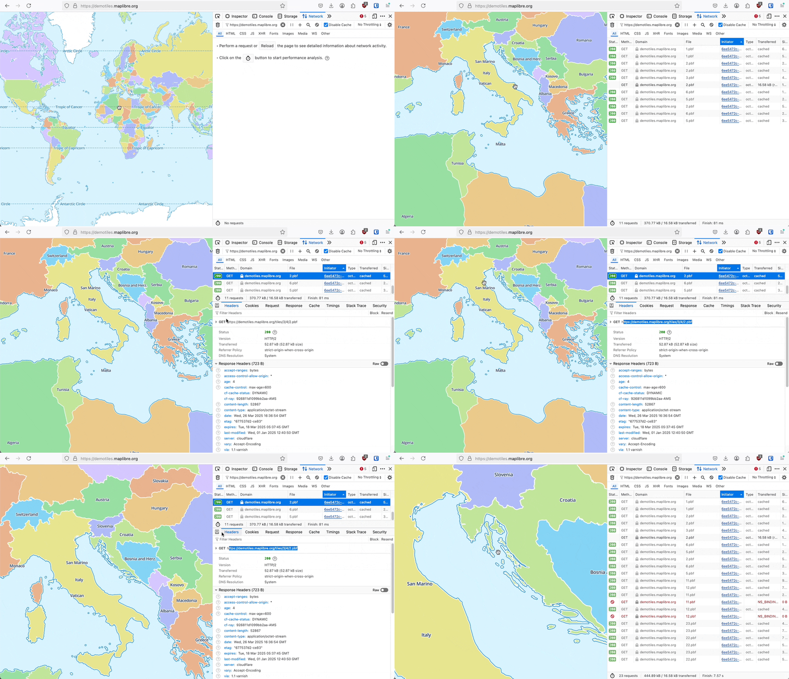
Look at the below GIF how more and more .pbf files are loaded when zooming or moving around the map.
6. 5 Vector Tile Format
Vector tiles do not use file formats like GeoJSON, FlatGeobuf, or GeoPackage. Those are excellent for data storage or file exchange, but not typically for the on-the-fly retrieval of map slices at each zoom level.
Instead, they are delivered in file formats like:
.pbf(Protocolbuffer Binary Format) – A commonly used, lightweight format..mvt(Mapbox Vector Tile) – A variant of PBF created by Mapbox with additional features, which is the industry standard today.
Mapping libraries (MapLibre, Mapbox GL JS, etc.) know how to parse that binary data to draw roads, buildings, water, and labels at the correct locations and style.
These are usually served by a Tile Server, which creates them on the fly from large geospatial datasets like OpenStreetMap's base map. We will shortly introduce you to Tile Servers and how they work in detail.
6.6 Different Tile Standards and Where Tiles Come From
When your mapping library fetches tiles, it often uses a specific tile standard to figure out how to form the {z}/{x}/{y} URLs or coordinates. You might see references to “Slippy Maps,” “TMS,” “WMTS,” or “OGC API Tiles.” These are different protocols or specifications that define exactly how tile coordinates are named and how they are requested.
Slippy Map Tiles (OpenStreetMap Style) - This is the most common implementation of the XYZ format pioneered and used by Google Maps. In this standard, the coordinate
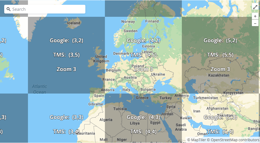
[0,0]is defined at the top-left corner of the map. This convention has become the default for many implementations today, but was never officially standardized.TMS (Tile Map Service) - The TMS standard was introduced to bring consistency to tile services. It is nearly identical to Slippy Map Tiles, except that
[0,0]is defined at the bottom-left corner of the map. Essentially, TMS is just Slippy Map Tiles with a flipped Y coordinate. This approach aligns better with traditional GIS software, though it never achieved widespread adoption.WMTS (Web Map Tile Service) - A standard from the OGC (Open Geospatial Consortium) where the URLs often look a bit more complex, with additional parameters like layer names, styles, or coordinate reference system info. Many desktop GIS tools or enterprise solutions use WMTS services, but it's less common in web applications.
OGC API Tiles - A newer OGC standard for tiles that builds on modern web concepts and RESTful patterns. It aims to standardize how you discover and request tiles from an API endpoint, but support for OGC API Tiles is still limited due to their relative newness.
Interactive Playground
For an interactive look at how tile coordinates work, visit Tiles à la Google Maps. This tool lets you inspect tile coordinates and see the differences between Slippy Map Tiles (Google) and TMS tile values, helping you understand how each system maps the world.
6.7 Tiling for Your Own Data
So far, we have described how base maps (like OpenStreetMap) use tiling. But you can also apply this same concept to your own large dataset. Instead of loading everything at once, divide your dataset into smaller tiles that load only when needed. This dramatically improves performance by displaying only the data relevant to the current viewport.
This is what we were leading up to when we said that "even Deck.gl will struggle to render everything in a single layer when dealing with datasets containing millions of points or files exceeding hundreds of megabytes".
7. Creating and Serving Vector Tiles
So, how do you actually generate and serve vector tiles? Here are three main ways.
7.1 Generating Tiles on Demand
In this approach, your complete dataset is stored in a database, usually PostgreSQL with the PostGIS extension to handle geospatial queries. When a user requests a tile (for example, zoom level 10, x=25, y=50), the server:
Finds all items within the tile’s geographic boundary (for example, roads, buildings, or points of interest).
Converts these items into vector shapes.
Packages them into a
.pbfor.mvtfile and sends it back to the user.
The biggest advantage of generating tiles on demand is that any changes to your data are visible immediately. You simply update the database, and fresh tiles are created for users in real time. However, this can put heavy load on your server and database when many users are zooming and panning at once. You can set up caching to reduce repeated work, but more about that later.
7.2 Pre-Generating All Tiles into a Single File (Using MBTiles)
Another approach is to create all the tiles in advance and store them in a single “tile package” file. A popular format is MBTiles, which is basically an SQLite database containing all your tiles for each zoom level.
You can use tools such as:
These tools can convert your source data (for example, GeoJSON) into an MBTiles file. Then you can upload that .mbtiles file to a hosting service (for example, AWS S3 or Cloudflare R2). Since MBTiles is just an SQLite database, you do not need to run a separate database server. A tile server can read from this file directly and respond to tile requests very quickly, because the tiles are already prepared.
The downside to pre-generation is that you must recreate the .mbtiles file every time your data changes. This process can take a long time if your dataset is large, making it less suitable if your data is updated often.
7.3 File-Based PMTiles
PMTiles (Protomaps) is a newer approach that stores your pre-generated vector tiles in a single file ``, similar to MBTiles. However, it arranges them so that the file can be read directly in a serverless way. In other words, your users’ browsers can request only the parts of the file they need (byte ranges) based on tile coordinates, without any custom server code.
Because of that, you can simply host the PMTiles file on a static file hosting service(AWS S3 or Cloudflare R2). The user’s browser will download the relevant tile data on its own, making the process very simple. Similarly to MBTiles, the main drawback is that you still have to regenerate the PMTiles file if your data changes, which may be slow for very large datasets.
7.4 Serving Your Tiles
PMTiles can be served directly, as long as the file is accessible over the internet. Tools like MapLibre can then fetch the vector tiles right from it.
If you decide to use PostgreSQL or MBTiles, you will need a Tile Server to stand between your map and your data. The tile server will read from your database or your MBTiles file and return the requested tiles to the browser. Many third-party services can do everything for you (just upload your dataset and off you go), but costs may go up as map traffic grows. You can also find open-source tile servers that handle database queries with little to no extra coding on your part.
Still, if you truly want to understand how vector tiles are made and delivered, it is worth learning how to set up a tile server using PostgreSQL. We will build one ourselves so you can see it in action. After that, we will look at different hosting services and self-hosted options, so you can decide which route fits your project best.
8. Building a Tile Server
Let's walk through the process of setting up a simple tile server.
Prerequisites
You should be comfortable with SQL databases and have some backend development experience. We will not go deep into backend coding because once you know how to store and retrieve data from the database, you understand the implementation process.
For this guide, we will use Docker to quickly create a PostgreSQL database with the PostGIS extension. If you prefer, you can set up PostgreSQL and PostGIS manually. From now on, we will refer to "PostgreSQL with PostGIS" simply as PostGIS.
To create a PostGIS database using Docker, run the following command:
docker run --name some-postgis -p 5432:5432 -e POSTGRES_PASSWORD=mysecretpassword -d postgis/postgis
This command will:
Download the official PostGIS Docker image if it is not already on your computer.
Start a PostGIS database container that you can access at
localhost:5432.Set the default username to postgres with the password mysecretpassword.
The Dataset
We will use a sample file called cities.geojson that contains six major cities from around the world:
{
  "type": "FeatureCollection",
  "features": [
    { "type": "Feature", "properties": { "city": "Paris" }, "geometry": { "coordinates": [2.3476, 48.8729], "type": "Point" }, "id": 0 },
    { "type": "Feature", "properties": { "city": "Berlin" }, "geometry": { "coordinates": [13.3346, 52.5506], "type": "Point" }, "id": 1 },
    { "type": "Feature", "properties": { "city": "Dubai" }, "geometry": { "coordinates": [55.3230, 25.2906], "type": "Point" }, "id": 2 },
    { "type": "Feature", "properties": { "city": "Seoul" }, "geometry": { "coordinates": [126.9386, 37.5502], "type": "Point" }, "id": 3 },
    { "type": "Feature", "properties": { "city": "Shanghai" }, "geometry": { "coordinates": [121.4904, 31.2123], "type": "Point" }, "id": 4 },
    { "type": "Feature", "properties": { "city": "Tokyo" }, "geometry": { "coordinates": [139.7003, 35.6761], "type": "Point" }, "id": 5 }
  ]
}
What We Want to Achieve
Our goal is to serve a dataset as vector tiles so that only relevant data is loaded based on the visible area of the map.
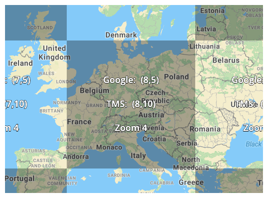
For example, a request to:
https://our-tile-server.com/4/8/5.mvt
should return an MVT file that contains only the cities inside that tile. At zoom level 4, tile x = 8, y = 5 covers most of Europe, returning just Paris and Berlin.
To understand which coordinates fall inside a tile at different zoom levels, check out MapTiler’s Tile Coordinates Guide.
We're choosing .mvt instead of .pbf because .mvt is more widely recognized and standardized across modern map libraries and tile servers.
Step 1: Create Your Table
In standard PostgreSQL, you define tables using data types like VARCHAR(200) and INTEGER. With PostGIS, you have extra spatial data types available. These include GEOMETRY and GEOGRAPHY.
For this project, we will use the GEOMETRY type, which is similar to the coordinate structure in GeoJSON. Our table will store the city names along with their geographical points (longitude and latitude).
Create the cities table with the following SQL command:
CREATE TABLE cities (
    id SERIAL PRIMARY KEY,
    name VARCHAR(150),
    geom GEOMETRY(Point, 4326)
);
In the code above, geom GEOMETRY(Point, 4326) defines a column that stores point data (longitude and latitude). The number 4326 tells the database which coordinate system to use. We will explain this more later.
It is common practice to name columns that use the
GEOMETRYdata type asgeom.
The GEOMETRY type supports several spatial data subtypes:
Point: Represents a single coordinate (for example, a city location).LineString: Represents a series of connected points, namely Polylines (for example, roads or rivers).Polygon: Represents an enclosed area (for example, city boundaries or lakes).MultiPoint,MultiLineString,MultiPolygon: These are collections of the above types.
If you are unsure what geometry types you will store in one column you can use the generic Geometry type:
    ...
    geom GEOMETRY(Geometry, 4326)
    ...
This allows the geom column to store any type of geometry!
About Coordinate Systems: WGS84 and Web Mercator
What does 4326 mean?
Many of us are familiar with the latitude and longitude system, based on WGS84 (EPSG:4326) standard. This system represents locations on Earth using a 3D globe model, which makes it very accurate for real-world data.
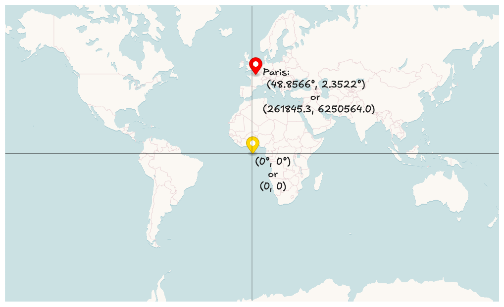
When we view maps online, we usually use a different system called Web Mercator (EPSG:3857). This system is designed for web maps because it works well for 2D mapping. However, Web Mercator distorts distances and areas, especially near the poles (Greenland looks bigger than Africa, while that isn't true). It uses meters as its unit.
For example, consider the position of Paris, France:
📍 WGS84 (EPSG:4326):
(48.8566°, 2.3522°)📍 Web Mercator (EPSG:3857):
(261845.3, 6250564.0)
Most online mapping platforms (like Google Maps, OpenStreetMap, and Mapbox) store geographic data in WGS84. But behind the scenes, they then convert the data into Web Mercator when rendering the map as 2D in the browser. This method keeps the data accurate while allowing fast and efficient rendering in the web. The same applies to MapLibre: it accepts data in WGS84 coordinates and later transforms them to Web Mercator when rendering.
Because of this, you will mostly work with WGS84 (EPSG:4326) . That is why we specified 4326 in our table:
geom GEOMETRY(Geometry, 4326)
Step 2: Inserting Data
PostGIS provides an easy way to insert GeoJSON data using the function ST_GeomFromGeoJSON().
Consider one feature from our dataset:
    //...
    {
      "type": "Feature",
      "properties": { "city": "Paris" },
      "geometry": { "coordinates": [2.3476, 48.8729], "type": "Point" },
      "id": 0
    }
    //...
ST_GeomFromGeoJSON() accepts only the geometry value. Other properties, like the city name, have to be inserted into separate columns.
Inserting GeoJSON Data into the cities Table
You can insert the GeoJSON data into the cities table with this SQL command:
INSERT
    INTO
    cities (name, geom)
VALUES
    (
        'Paris',
        ST_GeomFromGeoJSON('{"type":"Point","coordinates":[2.3476, 48.8729]}')
    ),
    (
        'Berlin',
        ST_GeomFromGeoJSON('{"type":"Point","coordinates":[13.3346, 52.5506]}')
    ),
    (
        'Dubai',
        ST_GeomFromGeoJSON('{"type":"Point","coordinates":[55.3230, 25.2906]}')
    ),
    (
        'Seoul',
        ST_GeomFromGeoJSON('{"type":"Point","coordinates":[126.9386, 37.5502]}')
    ),
    (
        'Shanghai',
        ST_GeomFromGeoJSON('{"type":"Point","coordinates":[121.4904, 31.2123]}')
    ),
    (
        'Tokyo',
        ST_GeomFromGeoJSON('{"type":"Point","coordinates":[139.7003, 35.6761]}')
    );
After running the query, your table should look like this:
| id | name | geom |
| 1 | Paris | POINT (2.3476 48.8729) |
| 2 | Berlin | POINT (13.3346 52.5506) |
| 3 | Dubai | POINT (55.323 25.2906) |
| 4 | Seoul | POINT (126.9386 37.5502) |
| 5 | Shanghai | POINT (121.4904 31.2123) |
| 6 | Tokyo | POINT (139.7003 35.6761) |
Step 3: Get Data
Now, using three values z = 4, x = 8, and y = 5, we want to get the coordinate data for Paris and Berlin. However, PostGIS does not understand XYZ tile values directly. Instead, PostGIS works with geometric shapes like points, polylines, and polygons.
Luckily, PostGIS has helper functions that let us convert tile values into a square polygon.
Step 3.1: Determine the Tile's Bounding Box
To get data from the right area, we first need to calculate the bounding box of the tile (z=4, x=8, y=5). A bounding box is simply a polygon that outlines the tile.
PostGIS has two useful functions for this:
ST_TileEnvelope(z, x, y)returns the bounding box of a tile at the given z, x, and y values, but returns it in Web Mercator (EPSG:3857).ST_Transform(geometry, 4326)converts the bounding box from Web Mercator (EPSG:3857) to WGS84 (EPSG:4326) (which uses latitude and longitude).
You can get the bounding box with this SQL query:
SELECT ST_Transform(ST_TileEnvelope(4, 8, 5), 4326);
The above query returns the polygon for the tile (z=4, x=8, y=5):
POLYGON ((0 40.979, 0 55.776, 22.499 55.776, 22.499 40.979, 0 40.979))
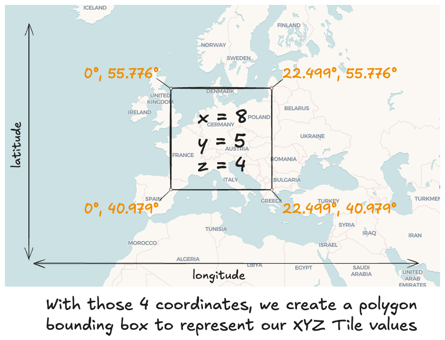
Now that we have the bounding box, we can use it to filter the cities in our cities table that are within this area.
Step 3.2: Retrieve Cities as GeoJSON
Mapbox Vector Tiles (MVT) is binary data, making it difficult to read the response.
Therefore, as an optional intermediate step, we can first fetch the data in human-readable GeoJSON format. This helps us verify that the data is being filtered correctly before moving on to the MVT format.
WITH tile_bbox AS (
    SELECT ST_Transform(ST_TileEnvelope(4, 8, 5), 4326) AS bbox
)
SELECT id, name, ST_AsGeoJSON(geom) AS geojson
FROM cities, tile_bbox
WHERE ST_Intersects(geom, bbox);
Here is what the query does:
WITH tile_bbox AS (...): Calculates the bounding box and saves it asbboxin a temporary table calledtile_bbox.SELECT id, name, ST_AsGeoJSON(geom) AS geojson: Gets theidandnameof each city and converts thegeomcolumn into GeoJSON format.FROM cities, tile_bbox: This is a cross join. It means we're combining every city in thecitiestable with the bounding box we calculated intile_bbox. We aren't specifying a normal join condition (like matching IDs); instead, we're just combining all the cities with the bounding box.WHERE ST_Intersects(geom, bbox): Only includes the cities that have geometry that intersects with the bounding box.
For visualisation, the cross join (FROM cities, tile_bbox) produces a temporary table like this:
| id | name | geojson | bbox |
| 1 | Paris | {"type":"Point","coordinates":[2.3476,48.8729]} | POLYGON ((0 40.979, 0 55.776, 22.499 55.776, 22.499 40.979, 0 40.979)) |
| 2 | Berlin | {"type":"Point","coordinates":[13.3346,52.5506]} | POLYGON ((0 40.979, 0 55.776, 22.499 55.776, 22.499 40.979, 0 40.979)) |
| 3 | Dubai | {"type":"Point","coordinates":[55.323,25.2906]} | POLYGON ((0 40.979, 0 55.776, 22.499 55.776, 22.499 40.979, 0 40.979)) |
| 4 | Seoul | {"type":"Point","coordinates":[126.9386,37.5502]} | POLYGON ((0 40.979, 0 55.776, 22.499 55.776, 22.499 40.979, 0 40.979)) |
| 5 | Shanghai | {"type":"Point","coordinates":[121.4904,31.2123]} | POLYGON ((0 40.979, 0 55.776, 22.499 55.776, 22.499 40.979, 0 40.979)) |
| 6 | Tokyo | {"type":"Point","coordinates":[139.7003,35.6761]} | POLYGON ((0 40.979, 0 55.776, 22.499 55.776, 22.499 40.979, 0 40.979)) |
After applying the filter with WHERE ST_Intersects(geom, bbox), only the cities that lie inside the bounding box are returned. The final result of the query returns:
| id | name | geojson |
| 1 | Paris | {"type":"Point","coordinates":[2.3476,48.8729]} |
| 2 | Berlin | {"type":"Point","coordinates":[13.3346,52.5506]} |
Great! We have now retrieved the data for the correct cities. Next, we will convert this data into Mapbox Vector Tile (MVT) format.
Step 3.3: Converting Data to MVT Format
Mapbox Vector Tile (MVT) is a compact binary format for geographic data. They are designed for fast rendering in maps. Unlike GeoJSON (which is human-readable and uses latitude/longitude), MVT files use binary encoding and a special tile coordinate system.
Each Vector Tile typically works within a space of 4096 x 4096—a size referred to as its extent. Instead of storing exact longitude and latitude values (e.g., 2.35°, 48.85°), MVT places data points within the tiles boundary (e.g., 1021x2039 relative to a tiles 4096x4096 space).
FYI: GeoJSON can only hold a single
FeatureCollection, or in other words, a single dataset like "cities". Meanwhile, MVT tiles can contain severalFeatureCollection, separated as an array of what they call "layers" (for example, one layer forcitiesand another forroads).
To see how the conversion works, let’s modify our query in two steps.
First, transform the geometry into tile coordinates:
WITH tile_bbox AS (
    SELECT ST_Transform(ST_TileEnvelope(4, 8, 5), 4326) AS bbox
)
SELECT
    id,
    name,
+    ST_AsMVTGeom(
+        geom,
+        bbox,
+        extent => 4096, -- The size the tile in pixels (commonly 256 or 4096)`
+        buffer => 256 -- Adds an optional buffer to handle feature clipping at tile edges
+    ) AS geom
FROM cities, tile_bbox
WHERE ST_Intersects(geom, bbox);
This query is very similar to the one in Step 3.2, except that it uses ST_AsMVTGeom() to change the geometries into the correct format for an MVT tile. We set the extent to 4096 pixels and add a buffer of 256 pixels. The buffer is useful because it reduces visual problems along the edges of each tile.
The result of this query would be:
| id | name | geom (In tile coordinates) |
| 1 | Paris | POINT (427 1911) |
| 2 | Berlin | POINT (2427 893) |
Here, you can see that the geometry values are no longer in latitude and longitude. Instead, they have been converted into positions that fit within a 4096 x 4096 grid.
To finish, we package the data into a valid binary MVT format using the ST_AsMVT() function:
WITH tile_bbox AS (
    SELECT ST_Transform(ST_TileEnvelope(4, 8, 5), 4326) AS bbox
)
+ SELECT ST_AsMVT(tile, 'cities', 4096) AS mvt
+ FROM (
    SELECT
        ST_AsMVTGeom(
            geom,
            bbox,
            extent => 4096, -- The size the tile in pixels (commonly 256 or 4096)`
            buffer => 256 -- Adds an optional buffer to handle feature clipping at tile edges
        ) AS geom,
        id,
        name
    FROM cities, tile_bbox
    WHERE ST_Intersects(geom, bbox)
+ ) AS tile;
Here’s how this query works:
We create an alias of the the previous query and name it as
tile.We then use
ST_AsMVT(tile, 'cities', 4096)to wrap the data into a binary MVT file.The second argument in
ST_AsMVT, namely'cities', is the layer name, and4096specifies once again the tile extent.
By running this query, you get a binary MVT tile as the result.
Now we can implement above query in for instance in an Express.js backend:
// server.js
app.get("/tiles/:z/:x/:y.mvt", async (req, res) => {
  const { z, x, y } = req.params;

  const sql = `
      WITH tile_bbox AS(
        ... ST_TileEnvelope($1, $2, $3) ...
      )
      SELECT ST_AsMVT ...
  `;

  const mvtBinary = await db.query(sql, [z, x, y]); // prepared statement

  res.setHeader("Content-Type", "application/vnd.mapbox-vector-tile");
  res.send(mvtBinary); // mvtData is a Buffer containing binary MVT
});
Now, Wwhen someone requests:
https://our-tile-server.com/4/8/5.mvt
JavaScript map libraries like Deck.gl's MVTLayer or Mapbox GL can display the returned data as map features right away.
Congratulations on building your first Tile Server! As explained from the start, we kept the backend code to a minimum to emphasize the strategy and process of managing data. Now that you've just learned how to store and retrieve data from your database, you're equipped to translate this knowledge into the backend functionality your project needs.
(Optional) Step 4: Simplifying or Clustering Geometry
In our current tile server setup, every tile sends all the data that lies within its area. This works well when you view the map at higher zoom levels because you see only a small part of the area. However, when a user zooms out completely (for example, at zoom level 0), one tile covers the entire world. In that situation, the tile includes the full data set, which makes the map appear very busy and hard to understand. Essentially, the benefit of using tiles is lost because you would be sending all the data at once.
To solve this problem, we can reduce the level of detail of our data at different zoom levels. This process is known as simplifying geometry or generalization. Simplifying geometry means reducing the complexity of vector shapes or combining several shapes together. For example:
When zoomed out, several points can be combined into one marker. As the user zooms in, these markers gradually separate into individual points.
A detailed polygon, such as an island with many intricate edges, can be simplified so that it has fewer edges.
By reducing the details, the map can load faster and display a clearer view when zoomed out.
We use the word "combining" in this text because it is easier to read. In technical terms, this process is called aggregation or clustering.
Real-World Examples
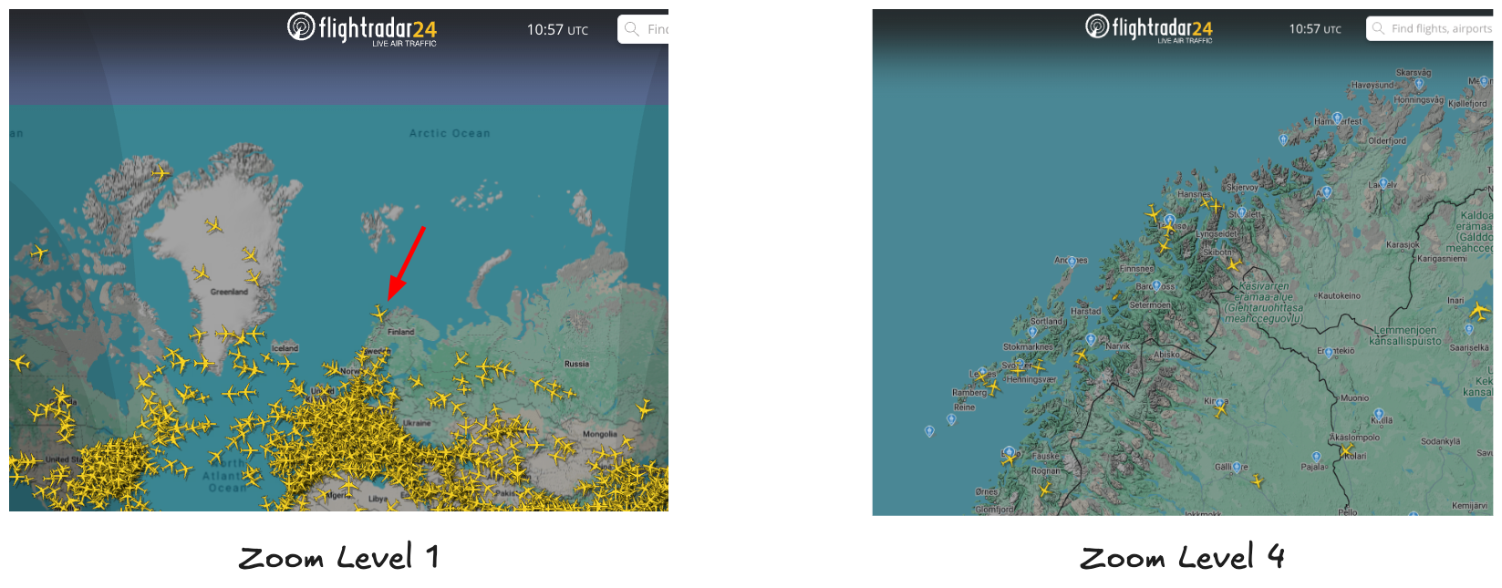
Flightradar24 is a website that displays real-time flights on a map. To avoid a crowded map at lower zoom levels and to save bandwidth, the website combines several nearby flights into one marker. In the image below, you see only one flight icon over northern Norway when the map is zoomed out. As you zoom in, more flight icons appear. This approach keeps detailed information hidden until a user chooses to zoom in.
Base Map Services such as Mapbox and Google Maps also avoid overloading a single tile. They use rules to decide which features appear at different zoom levels. For example, a rule might state that only main highways are shown when the map is zoomed out, and local roads are added as the user zooms in further.
How to Implement Geometry Simplification
The function ST_AsMVTGeom() already reduces some detail in polylines and polygons. However, this built-in simplification might not be enough, and it does not work for points. (Sources: 1, 2, 3)
We can improve the process by using additional functions:
Use
ST_Simplify()to reduce the shape complexity of polylines and polygons.Use a combination of
ST_ClusterWithin,ST_Collect, andST_Centroidto combine points that are close together.
The code snippet below shows how to integrate ST_Simplify into our existing query. In this example, the simplification is applied before the call to ST_AsMVTGeom:
WITH tile_bbox AS (
    SELECT
        ST_Transform(ST_TileEnvelope(4, 8, 5), 4326) AS bbox,
)
SELECT ST_AsMVT(tile, 'cities', 4096) AS mvt
FROM (
    SELECT
        ST_AsMVTGeom(
+            ST_Simplify(
+                geom,
+                CASE
+                    WHEN 5 <= 3 THEN 0.01
+                    WHEN 5 <= 10 THEN 0.005
+                    WHEN 5 <= 15 THEN 0.001
+                    ELSE 0
+                END
+            ),
            bbox,
            extent => 4096,
            buffer => 256
        ) AS geom,
        id,
        name
    FROM cities, tile_bbox
    WHERE ST_Intersects(geom, bbox)
) AS tile;
In this example, the value 0.01 is the tolerance value. This means that any detail smaller than 0.01 degrees is removed. The larger the value, the more aggressive the simplification.
In our current dataset, which is based only on points, this above change won't actually have have any effect, since ST_Simplify only works on Polylines and Polygons. However, you should understand the concept from this example.
If you decide to implement the functions ST_ClusterWithin, ST_Collect, and ST_Centroid, to actually have an impact on points, the query will become more complex. This is because you must create several alias queries to process the data in stages:
ST_ClusterWithin: This function groups together points that are close to each other and returns these points as an array.
ST_Collect: This function combines multiple geometries into a single MultiPoint collection, which is required for the next step.
ST_Centroid: This function calculates the center of mass of a geometry collection, allowing you to place one marker to represent multiple points.
Inspecting the MVT Binary Data
Libraries like Deck.gl's MVTLayer use loaders.gl to fetch and parse MVT data. The loader retrieves the binary MVT file and passes it through an MVT parser.
The parser converts the MVT data to GeoJSON by scaling the tile coordinates to a range between 0 and 1. For example:
import { MVTLoader } from "@loaders.gl/mvt";
import { parse } from "@loaders.gl/core";

app.get("/tiles/:z/:x/:y.mvt", async (req, res) => {
  const { z, x, y } = req.params;

  const sql = `
      WITH tile_bbox AS(
        ... ST_TileEnvelope($1, $2, $3) ...
      )
      SELECT ST_AsMVT ...
  `;

  const mvtBinary = await db.query(sql, [z, x, y]); // prepared statement

  const mvtAsGeoJSON = await parse(mvtBinary, MVTLoader, {
    mvt: {
      layers: ["cities"],
      coords,
    },
  });

  console.log(mvtAsGeoJSON); // The result is a JavaScript array of GeoJSON features.
});
When you log mvtAsGeoJSON, you see an array of GeoJSON features with coordinates scaled between 0 and 1, which are their coordinates within the tile. For example:
[
    {
      type: "Feature",
      geometry: {
        type: "Point",
        coordinates: [0.0987, 0.4417],
      },
      properties: {
        id: 1,
        name: "Paris",
        layerName: "cities",
      },
    },
    {
      type: "Feature",
      geometry: {
        type: "Point",
        coordinates: [0.561, 0.2064],
      },
      properties: {
        id: 2,
        name: "Berlin",
        layerName: "cities",
      },
    },
];
9. Tile Server Best Practices
You now understand the basics of a Tile Server, but there are still some important gotchas that you should learn.
9.1 Strategies for Inserting Large Datasets into PostGIS
When your data source has millions of records or files larger than 100 MB, you should not use the insert approach from "Section 8 - Step 2: Inserting Data" with ST_GeomFromGeoJSON. For instance, if you ran that insert query in Node.JS, loading an entire large file into Node.js memory can crash your backend. Instead, you want to read large files in small parts or use tools optimized for this. Below are some strategies:
Using PostgreSQL's COPY Statement
You can use PostgreSQL's COPY statement to import data efficiently. Since COPY supports a limited number of file formats (e.g., CSV), you’ll first need to convert your data into a CSV file with columns like:
| id | name | geojson |
| 1 | Paris | {"coordinates":[2.3476,48.8729],"type":"Point"} |
| 2 | Berlin | {"coordinates":[13.3346,52.5506],"type":"Point"} |
| 3 | Dubai | {"coordinates":[55.3230,25.2906],"type":"Point"} |
| ... | ... | ... |
Then use the COPY command to import the data:
COPY cities(id, name, geom)
FROM '/path/to/cities_geojson.csv'
DELIMITER ','
CSV HEADER
WITH (
  FORMAT 'csv',
  TRANSFORM (
    geom FROM (geojson) USING ST_GeomFromGeoJSON(geojson)
  )
);
You can run this command from the psql command line. You can also run it in Node.js, but be careful to use streams. Streams reads large files incrementally, instead of loading them fully into memory (Here is an example).
In Node.js
In Node.js, you can use loaders.gl to process data in streams. Not all loaders support streaming, but some do. This method allows you to load data incrementally without using too much memory. Here is an example using FlatGeobuf:
import {FlatGeobufLoader} from '@loaders.gl/flatgeobuf';
import {loadInBatches} from '@loaders.gl/core';

const batches = await loadInBatches('data.fgb', FlatGeobufLoader);

for await (const batch of batches) {
  // batch.data will contain a number of rows
  for (const feature of batch.data) {
    console.log("Type", feature.geometry.type) // "Point"
    console.log("Coordinates", feature.geometry.coordinates) // [2.3476, 48.8729]
    // Store in Database
  }
}
Using ogr2ogr
Another method recommended in the official PostGIS documentation is to use ogr2ogr. This is a command-line tool that helps you insert geospatial data into a database.
ogr2ogr is part of the GDAL (Geospatial Data Abstraction Library). Once you install GDAL, you can load any geospatial data format into PostGIS. Here is an example using GeoJSON:
ogr2ogr -f "PostgreSQL" PG:"host=localhost port=5432 dbname=postgres user=postgres password=mysecretpassword" "cities.geojson"
Let’s explain the command:
-f "PostgreSQL"tells ogr2ogr that the output format is a PostgreSQL database.PG:"..."is the connection string with your database credentials (change as needed)."cities.geojson"is the source file you want to import.
By default, ogr2ogr will insert data into a table named after your input file (for example, cities). If the table does not exist, it creates one. It will also try to map properties to matching column names automatically.
You can change this behavior by specifying the table name and mapping columns with the -sql flag:
ogr2ogr ... -sql "SELECT city AS city_name FROM cities"
This command then results in the our table looking like this instead:
| id | name | geom | city_name |
| 1 | POINT (2.3476 48.8729) | Paris | |
| 2 | POINT (13.3346 52.5506) | Berlin | |
| 3 | POINT (55.323 25.2906) | Dubai | |
| 4 | POINT (126.9386 37.5502) | Seoul | |
| 5 | POINT (121.4904 31.2123) | Shanghai | |
| 6 | POINT (139.7003 35.6761) | Tokyo |
9.2 Improved Security with Tiles
Using Vector Tiles provides better security compared to rendering the entire dataset directly. For example, if you display your entire dataset in a GeoJSON file and render it on a Deck.gl layer, anyone viewing your website could easily download the entire dataset. But with vector tiles, the situation is different: you only send the necessary data required for the user's current view.
This approach is especially important when your data is valuable to your business or provides a competitive advantage.
To ensure the effectiveness of this security measure, you need to:
Simplify or cluster your tiles: Simplify or cluster your tiles so that the complete data is only available when a user requests the more detailed (or "zoomed in") tiles.
Rate-limit tile requests: By restricting the number of tile requests a user can make in a given time, you prevent rapid downloading of large amounts of data.
At first glance, an attacker might argue, "Tiles only slow me down. I can still download everything!" However, when your data is simplified at lower zoom levels and you enforce strict rate limits, extracting the entire dataset becomes very difficult.
Let's see why with a practical example: If you allow users to zoom in up to zoom level 14, there are more than 350.000.000 possible tiles (as explained here). If you rate-limit the number of tile requests a user can make—for example, to 10.000 tiles per hour, which is quite generous—it would take an attacker many months to download the complete detailed dataset. During this time, your data would likely change, forcing the attacker to start all over again. Additionally, you would probably notice if a user (for example, named "NotAScraper123") is repeatedly reaching the rate-limit.
9.3 Caching for Performance
Currently, every time someone requests a Tile from the URL like https://our-tile-server.com/4/8/5.mvt, the server runs a new database query, even if the data has not changed. If hundreds or thousands of users request the same tile at the same time, it can put extra load on your database.
Even if the data updates every 30 seconds, many users may request the same data repeatedly within that timeframe, which also adds unnecessary strain.
To improve performance, consider the following caching strategies:
Backend Caching: Use tools like Redis or Memcached to store tile data temporarily so the database does not process the same query repeatedly. (Note: The server still receives and processes every request.)
CDN Caching: Services such as Cloudflare can completely offload requests from your server by caching the tiles. The CDN will serve the cached tile until the cache expires or is purged.
Client-Side Caching: Use HTTP headers (for example,
Cache-Control: max-age=30, public) so that browsers reuse tiles, which reduces the number of requests to your server.
10. Choosing an optimal Architecture for Delivering Your Map Data
Now that you have learned the fundamentals of heavy map visualizations and how tile servers work, it is time to decide on the best way to deliver both your base map and your own geospatial data. In this section, we discuss different approaches so that you can choose the solution that works best for your application—both now and as your project grows.
10.1 Open-Source Solutions
We already touched upon PMTiles (Protomaps) and MBTiles. These formats are popular because they allow you to convert your data, like a base map or your own geospatial data, into a single file that works with many open-source tile servers such as:
These solutions either work directly by accepting your .pmtiles or .mbtiles file, or by connecting to a PostGIS database that has been populated by those files (or other methods). You can also choose to avoid a tile server altogether by hosting a .pmtiles file on a static file service like AWS S3 or Cloudflare R2.
You may also write your own backend code to serve tiles, now that you understand the basics. However, for serving base maps, we recommend using one of the many reliable open-source solutions rather than building your own from scratch. For instance, serving the OpenStreetMap base map requires more than just tiling and simplifying some vector shapes.
Downloading Base Maps
Remember that both base maps and your own data are essentially vector shapes. Base maps, however, are pre-made datasets that can be very large (up to 150 GB). Here are two popular open-source base maps that you can use with any of the above approaches:
OpenStreetMap (OSM): The most detailed and widely used open-source map. You can download the data from sources such as PlanetOSM, MapTiler Planet Data, or Geofabrik. (Always include an "© OpenStreetMap" label when you use this map.)
Natural Earth Data: A simplified global map that is usually less than 1 GB. This map has fewer details and does not require any copyright attribution, even for commercial use.
10.2 Ready-to-Use Services
If you do not want to manage your own tile server or backend for serving a base map and your own geospatial data, you can use ready-to-use services.
| Service Name | Base Map Details | Custom Data Hosting & Serving |
| Google Maps | Classic maps with a free tier of 100.000 requests; costs can be high as your app grows, hence why a lot of developers avoid it. | You can add a custom data layer with CSV files up to 2000 rows; handling larger datasets may be limited. |
| Carto | Free for non-commercial projects. | ❌ |
| OpenFreeMap | Open-source and free, but may not work well for very high traffic. | ❌ |
| Mapbox | Popular base maps with a free tier of 50.000 requests; widely used by developers. | Supports various file formats through Mapbox Studio (up to 300MB) or Mapbox Tiling Service (up to 25GB). |
| Maptiler | Offers a free tier of 100.000 requests, with a slight reduction in delivery speed. | With Maptiler Geodata Hosting, you can upload datasets (GeoJSON, GeoPackage, etc.) up to 100GB and serve them as tiles. |
| Stadia Maps | Free for non-commercial projects; only $20 1.000.0000 requests, making it the cheapest for high traffic apps. | ❌ |
10.3 Our Recommendations
Before diving into the specific recommendations, remember that we have already discussed MapLibre as a powerful and flexible frontend library for building interactive maps. No matter which backend architecture you choose to serve your base maps and vector data, MapLibre integrates seamlessly with these solutions, making it your frontend library of choice for a smooth and efficient mapping experience.
Base Maps
For most projects, we suggest starting with services like Maptiler or Mapbox. They offer a free tier (50.000 to 100.000 requests per month) that works well even for commercial applications. As your application grows, you can explore alternatives such as Stadia Maps or even consider self-hosting using PMTiles on a platform like Cloudflare, which can significantly reduce costs.
Your Own Vector Data
For custom geospatial data, it may be tempting to use ready-made services for quick prototypes. However, using these services may lock you quickly into their ecosystem. We recommend building your own backend code using a PostGIS database to query your own tiles and data. Also, you likely already have some backend code with a database to manage authentication and user data, so adding tile functionalities should be straight forward.
Summary
Let's summarize the key points covered in this guide:
Geospatial Data Basics:
Data is tied to specific locations on Earth.
Uses vector shapes: points, polylines, and polygons.
Enables functions like finding nearby places, tracking movement, creating heatmaps, and setting up geofences.
Base Maps and Data Sources:
A base map is the background layer with roads, landmarks, and other details.
You can add your own geospatial data (like restaurant locations or delivery routes) on top of the base map.
Data can come from internal teams, external providers, or public datasets.
Geospatial Data Formats:
Vector formats: GeoJSON, Shapefiles, FlatGeobuf, GeoPackage.
Raster formats: Satellite images, GeoTIFFs, JPEGs, PNGs.
Tabular formats: CSV files or spreadsheets with location information.
Interactive Maps with JavaScript Libraries:
Popular libraries include MapLibre, Google Maps API, Mapbox GL JS, Leaflet, and OpenLayers.
MapLibre is recommended for its flexibility, performance, and open-source benefits.
Heavy Data Visualization:
- Tools like Deck.gl help render large numbers of data points efficiently using WebGL and a layer-based approach.
Tiling:
Tiling divides a large map into smaller, manageable squares (tiles) that load as needed.
Tiles are identified by XYZ coordinates, which change with zoom levels.
Both raster and vector tiles are used to display maps efficiently.
Creating and Serving Vector Tiles:
Methods include generating tiles on demand from a PostGIS database, pre-generating tiles (MBTiles), or using PMTiles.
Tiles are packaged in compact binary formats (like .mvt) to improve loading and rendering speed.
Tile Server Best Practices:
Use efficient methods (such as PostgreSQL’s COPY or ogr2ogr) for handling large datasets.
Enhance security by simplifying or clustering data and rate-limiting tile requests.
Improve performance with backend, CDN, and client-side caching.
Architecture Options:
Open-Source Solutions: Use formats like PMTiles/MBTiles with open-source tile servers (Martin, tileserver-gl, Geoserver) or host your own file on a service like AWS S3 or Cloudflare R2.
Ready-to-Use Services: Consider services such as Google Maps, Mapbox, Maptiler, or Stadia Maps for both base maps and vector data hosting.
Our Recommendation: For long-term flexibility and cost control, consider building your own backend tile server (using PostGIS) for your custom data while relying on established services for base maps.
Subscribe to my newsletter
Read articles from Advena directly inside your inbox. Subscribe to the newsletter, and don't miss out.
Written by
