📚 What is Supervised Learning?
 Rohit Ahire
Supervised Learning in Python — Regression vs Classification with Code & Diagrams
🔍 Introduction
If you’ve ever used Spotify recommendations, email spam filters, or price predictions for used cars, you’ve experienced Supervised Learning in action.
But what exactly is supervised learning?
How does it work?
And can you build your own supervised learning model — even as a beginner?
Let’s break it all down — step-by-step — with real-world analogies, Python code, and clear visual intuition.
📘 Definition (ISLR Reference)
From “An Introduction to Statistical Learning” (ISLR):
Supervised Learning is the problem of inferring a function from labeled training data, consisting of input-output pairs.
In simpler terms:
🧠 In plain English: You teach a machine using labeled examples, and it learns to make predictions on new data.
🔁 Real-Life Examples
| Scenario | Input (X) | Output (Y) |
| Email Spam Filter | Email text | Spam / Not spam |
| House Price Prediction | Size, Location, Bedrooms | Price in dollars |
| Resume Shortlisting | Resume features | Hire / No Hire |
| Spotify Recommendations | Your listening history | Songs you’ll like |
In each case:
The input data is something we know
The output (label) is something we want to predict
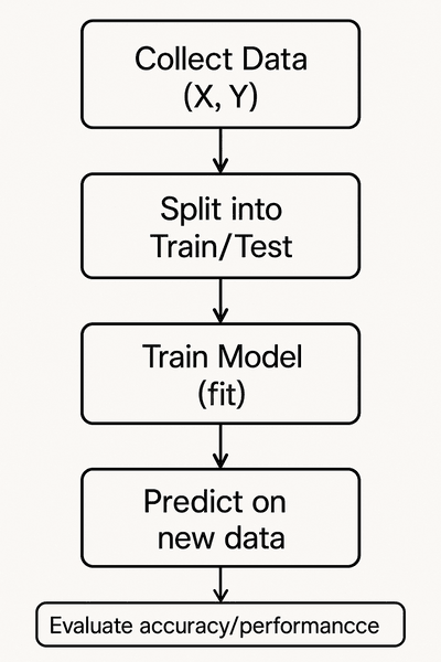
🛠️ Supervised Learning Process (Simple Flowchart)
📊 Types of Supervised Learning Tasks
There are two main types:
| Task Type | Description | Output Type |
| Regression | Predicts a continuous value | e.g., price = $220,000 |
| Classification | Predicts a category/class | e.g., spam or not spam |
🎯 What is Regression?
📘 Definition:
Regression is a type of supervised learning where the goal is to predict a continuous numerical value based on input features.
In simpler words:
Given some known information (like the size of a house), we want to predict a value (like its price).
🔍 Real-World Examples:
| Input (Features) | Output (Target Value) |
| Hours studied | Exam score (0–100) |
| House size & location | Price in dollars |
| Years of experience | Salary estimate |
| Temperature | Ice cream sales |
📈 What Regression Does:
Regression learns the relationship between features and outcomes by fitting a function (often a line, curve, or surface) that minimizes the difference between the actual and predicted values.
Imagine drawing the best-fit line through a cloud of data points.
🧪 Visual Example:
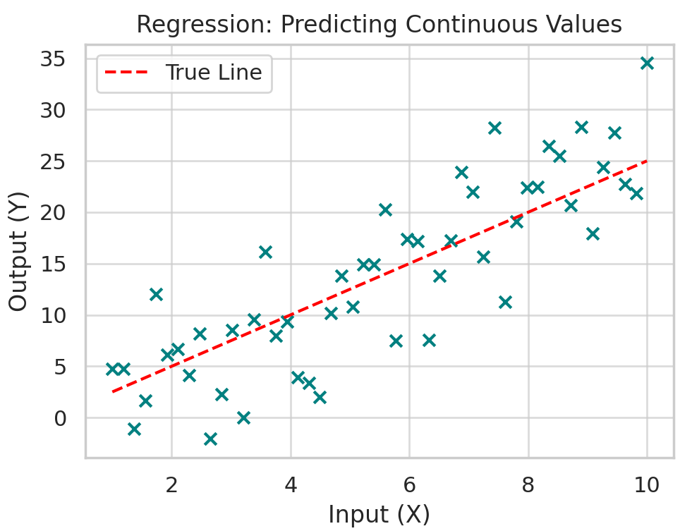
This chart shows how regression fits a line through noisy data to predict a continuous value.
The red dashed line represents the true underlying pattern, and the dots are real-world observations with some noise.
🧠 When to Use Regression:
When your target is numeric and continuous
You care about magnitude or value (not just category)
You want to estimate, not classify
🧪 Code for Linear Regression:
import numpy as np
import matplotlib.pyplot as plt

x = np.linspace(1, 10, 50)
y = 2.5 * x + np.random.randn(50) * 5  # Add noise

plt.scatter(x, y, color='teal')
plt.plot(x, 2.5 * x, color='red', linestyle='--', label="True Line")
plt.title("Regression: Predicting Continuous Values")
plt.xlabel("Input (X)")
plt.ylabel("Output (Y)")
plt.legend()
plt.show()
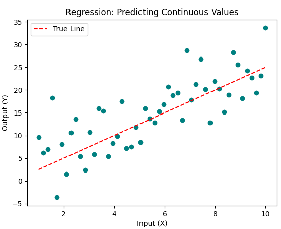
Output:
📊 Evaluation Metrics:
Mean Squared Error (MSE): average of squared differences between actual and predicted values
R² Score: how much of the variance is explained by the model
🧩 What is Classification?
📘 Definition:
Classification is a supervised learning technique where the goal is to assign input data to predefined categories or labels.
Instead of predicting a number, it decides:
“Which group does this belong to?”
🧠 Real-World Examples:
| Input | Output Class |
| Email content | Spam / Not spam |
| Tumor features | Benign / Malignant |
| Social media post | Positive / Neutral / Negative |
| Animal image | Dog / Cat / Rabbit |
🎯 What Classification Does:
It learns decision boundaries that separate different classes in the feature space.
Think of drawing a line (or curve) that separates apples from oranges based on color and size.
🧪 Visual Example:
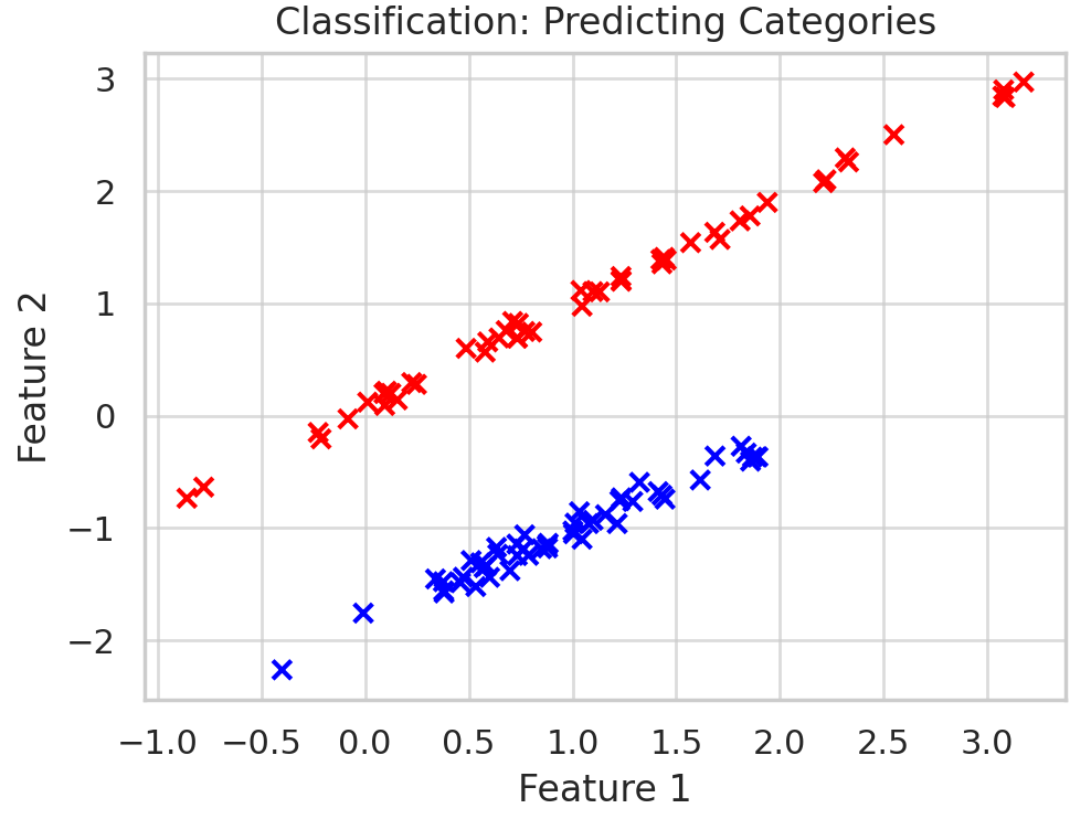
In the chart above:
Two features (x and y) describe each point
The red and blue dots represent two different classes
The model learns to draw a boundary line that separates them
🧪 Classification Code (Logistic Regression)
from sklearn.datasets import make_classification
import matplotlib.pyplot as plt

X, y = make_classification(n_samples=100, n_features=2,
                           n_redundant=0, n_informative=2,
                           n_clusters_per_class=1, random_state=42)

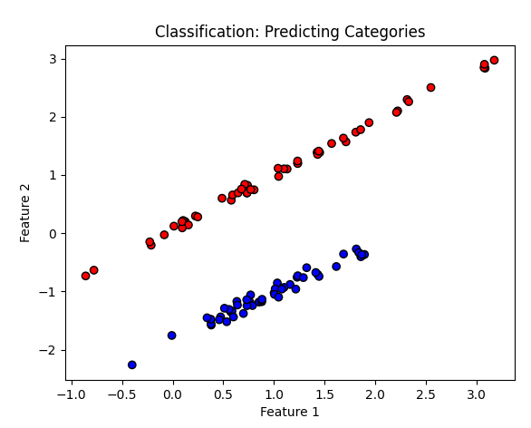
plt.scatter(X[:, 0], X[:, 1], c=y, cmap='bwr', edgecolors='k')
plt.title("Classification: Predicting Categories")
plt.xlabel("Feature 1")
plt.ylabel("Feature 2")
plt.show()
📊 Evaluation Metrics:
Accuracy: % of correctly predicted classes
Precision/Recall/F1-Score: used for imbalanced datasets
Confusion Matrix: shows true vs predicted class breakdown
🧪 Example: Student Exam Data
Imagine you're working with a dataset of students that includes:
Hours_StudiedSleep_HoursExam_Score
You want to:
Regression: Predict the exact exam score
Classification: Predict whether the student will pass or fail (based on score ≥ 50)
🧠 Step-by-Step Breakdown:
We’ll:
Create sample data
Train a regression model to predict score
Train a classification model to predict pass/fail
Compare results
✅ Code: Combined Regression + Classification
import pandas as pd
import numpy as np
import matplotlib.pyplot as plt
from sklearn.linear_model import LinearRegression, LogisticRegression
from sklearn.model_selection import train_test_split
from sklearn.metrics import mean_squared_error, accuracy_score, confusion_matrix, ConfusionMatrixDisplay

# 🎯 Step 1: Create sample data
np.random.seed(42)
n = 100
hours_studied = np.random.uniform(1, 10, n)
sleep_hours = np.random.uniform(4, 9, n)
exam_score = 5 * hours_studied + 2 * sleep_hours + np.random.normal(0, 5, n)
passed = (exam_score >= 50).astype(int)

# DataFrame
df = pd.DataFrame({
    "Hours_Studied": hours_studied,
    "Sleep_Hours": sleep_hours,
    "Exam_Score": exam_score,
    "Passed": passed
})

# 🎯 Step 2: Prepare features and targets
X = df[["Hours_Studied", "Sleep_Hours"]]
y_reg = df["Exam_Score"]
y_clf = df["Passed"]

# 🎯 Step 3: Train/Test split
X_train, X_test, y_reg_train, y_reg_test, y_clf_train, y_clf_test = train_test_split(
    X, y_reg, y_clf, test_size=0.2, random_state=42
)

# 🎯 Step 4: Train regression model
reg_model = LinearRegression()
reg_model.fit(X_train, y_reg_train)
reg_preds = reg_model.predict(X_test)

# 🎯 Step 5: Train classification model
clf_model = LogisticRegression()
clf_model.fit(X_train, y_clf_train)
clf_preds = clf_model.predict(X_test)

# 🎯 Step 6: Evaluate
reg_mse = mean_squared_error(y_reg_test, reg_preds)
clf_acc = accuracy_score(y_clf_test, clf_preds)

print(f"📊 Regression - Mean Squared Error: {reg_mse:.2f}")
print(f"📊 Classification - Accuracy: {clf_acc:.2%}")

# 🎯 Step 7: Visualize results

plt.figure(figsize=(14, 6))

# 📈 Subplot 1: Regression predictions vs actual
plt.subplot(1, 2, 1)
plt.scatter(range(len(y_reg_test)), y_reg_test, label="Actual", color='blue')
plt.scatter(range(len(y_reg_test)), reg_preds, label="Predicted", color='red', alpha=0.6)
plt.title(f"Regression: Predicting Exam Scores\nMSE = {reg_mse:.2f}")
plt.xlabel("Test Sample Index")
plt.ylabel("Exam Score")
plt.legend()

# 📊 Subplot 2: Classification confusion matrix
plt.subplot(1, 2, 2)
cm = confusion_matrix(y_clf_test, clf_preds)
disp = ConfusionMatrixDisplay(confusion_matrix=cm, display_labels=["Fail", "Pass"])
disp.plot(ax=plt.gca(), cmap='Blues', values_format='d')
plt.title(f"Classification: Pass/Fail\nAccuracy = {clf_acc:.2%}")

plt.tight_layout()
plt.show()
Output:
📊 Regression - Mean Squared Error: 16.66
📊 Classification - Accuracy: 100.00%
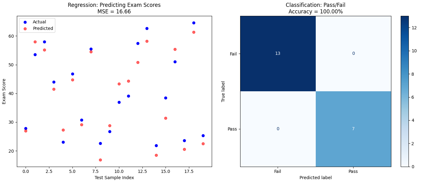
📉 In the left graph:You can see how close the red dots (predicted) are to the blue dots (actual exam scores). This is the goal of regression — accurate numerical predictions.
📊 In the right graph:The confusion matrix shows how well the classifier distinguished pass/fail outcomes. A perfect model predicts all correctly — like in this case.
✅ Summary
| Term | Meaning |
| Supervised Learning | Learning from labeled data |
| Input (X) | Known features |
| Output (Y) | Target variable |
| Regression | Continuous prediction |
| Classification | Category prediction |
| Fit | Learn pattern from data |
| Predict | Apply pattern to new data |
📘 This post is based on concepts from the book Introduction to Statistical Learning (ISLP) and adapted for practical implementation in Python.
🔁 What’s Next?
Coming up:
🧠 Unsupervised Learning Explained — Clustering and Dimensionality Reduction
🤖 Reinforcement Learning — How AI learns like humans
🧪 Visual Guide to All ChatGPT Models with Benchmarks
Subscribe to my newsletter
Read articles from Rohit Ahire directly inside your inbox. Subscribe to the newsletter, and don't miss out.
Written by
