Day 8: Polynomial Regression – Predicting Non-Linear Relationships
 Saket Khopkar
Till now, things were simple!!
All relationships were in straight line, so it was pretty easy to take certain decisions. Later we learned how Multiple Linear Regression (MLR) models relationships where the effect of independent variables is linear.
But what if the relationship between variables isn’t a straight line? 🤔
Let me give you some prominent examples:
Predicting population growth – It doesn’t increase at a fixed rate, it accelerates over time.
Stock prices – They rise and fall in curved trends.
House prices – Small houses increase in price slowly, but larger houses increase exponentially in value.
This is where Polynomial Regression comes in the picture!
Introduction
Polynomial Regression is an extension of Linear Regression that models curved relationships between variables.
Instead of fitting a straight line, Polynomial Regression fits a curved line to the data.
Imagine (Just Imagine for now) you are a business owner and you intend to track your revenue for the last 10 years.
| Year | Revenue ($) |
| 1 | 5 |
| 2 | 8 |
| 3 | 12 |
| 4 | 20 |
| 5 | 35 |
| 6 | 60 |
| 7 | 95 |
| 8 | 150 |
| 9 | 230 |
| 10 | 350 |
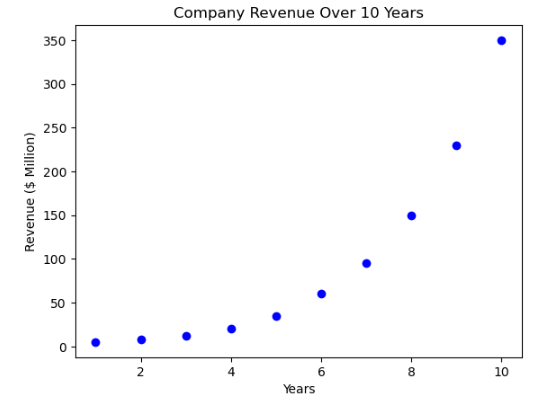
A successful business it seems!! If you plot this data, you don’t get a straight line instead, you might notice revenue accelerates over time.
When to use Polynomial Regression?
Now that you are clear with the basic what exactly Polynomial Regression is, let us have a look at when should you use this concept.
We use Linear Regression when the relationship between variables is straight (e.g., salary vs experience). We use Polynomial Regression When the relationship is curved (e.g., revenue vs time, stock price trends, temperature variations). This is the basic difference. Let us have a look at another example.
You must have seen cars, OFCOURSE you must have seen cars. Well when some obstacle comes in front of the car suddenly, the driver applies for brakes. Cutting the crap aside, we are going to imagine a scenario of Car’s Braking Distance for our example as below:
| Speed (km/hr) | Braking Distance (m) |
| 20 | 5 |
| 40 | 20 |
| 60 | 45 |
| 80 | 80 |
| 100 | 125 |
Now, a Linear Model would assume braking distance increases steadily with speed. Thats not practically possible isn’t it? But braking increases exponentially because higher speeds require significantly more distance to stop.
Mathematical Intuitions
Well Maths isn’t my forte, yet I will try my best.
You might recognize this equation from previous blogs:

This is for simple Linear Equation which draws a straight line.
As this is a Mathematical section, lets make things a bit complicated:
We introduce higher-degree terms (squared, cubed, etc.):

Where,
X² allows for curvature.
X³ and further allow for more flexibility.
Here is one of the example:
A quadratic model (degree = 2) may look like: Revenue = 2 + (5 X Year) + (3 X Year²)
Similarly, a cubic model (degree = 3) should be like : Revenue = 2 + (5 X Year) + (3 X Year²) + (0.5 X Year³)
And so on.
Higher-degree polynomials capture complex patterns as required.
Practical Demonstration
For our practical demonstaration, let’s build a Polynomial Regression model to predict revenue growth over 10 years.
import numpy as np
import pandas as pd
import matplotlib.pyplot as plt
from sklearn.preprocessing import PolynomialFeatures
from sklearn.linear_model import LinearRegression

# Creating dataset
years = np.array([1, 2, 3, 4, 5, 6, 7, 8, 9, 10]).reshape(-1, 1)
revenue = np.array([5, 8, 12, 20, 35, 60, 95, 150, 230, 350])

# Plot raw data
plt.scatter(years, revenue, color="blue")
plt.xlabel("Years")
plt.ylabel("Revenue ($ Million)")
plt.title("Company Revenue Over 10 Years")
plt.show()

A clear observation that the revenue tends to follow an exponential growth pattern, not necessarily a straight line.
Lets train the model using the baseline:
# Train Linear Regression model
linear_model = LinearRegression()
linear_model.fit(years, revenue)

# Predict using Linear Regression
linear_predictions = linear_model.predict(years)

# Plot Linear Regression results
plt.scatter(years, revenue, color="blue", label="Actual Revenue")
plt.plot(years, linear_predictions, color="red", label="Linear Regression")
plt.xlabel("Years")
plt.ylabel("Revenue ($ Million)")
plt.legend()
plt.title("Linear Regression Fails to Capture the Curve")
plt.show()

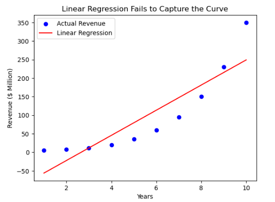
Issue: The straight-line model doesn’t match the real data well.
To capture so, we will be needing the model to trained to the degree 2
# Transform data into polynomial features (degree=2)
poly = PolynomialFeatures(degree=2)
X_poly = poly.fit_transform(years)

# Train Polynomial Regression model
poly_model = LinearRegression()
poly_model.fit(X_poly, revenue)

# Predict using Polynomial Regression
poly_predictions = poly_model.predict(X_poly)

# Plot results
plt.scatter(years, revenue, color="blue", label="Actual Revenue")
plt.plot(years, poly_predictions, color="green", label="Polynomial Regression (Degree 2)")
plt.xlabel("Years")
plt.ylabel("Revenue ($ Million)")
plt.legend()
plt.title("Polynomial Regression Fits the Curve Better")
plt.show()

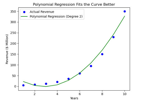
So, the verdict is : Polynomial Regression fits the curve better.
Lets Evaluate our model:
from sklearn.metrics import mean_squared_error, r2_score

# Calculate R² scores
linear_r2 = r2_score(revenue, linear_predictions)
poly_r2 = r2_score(revenue, poly_predictions)

print(f"Linear Regression R² Score: {linear_r2:.2f}")
print(f"Polynomial Regression R² Score: {poly_r2:.2f}")
Linear Regression R² Score: 0.80
Polynomial Regression R² Score: 0.98
So, we can cleary see that Polynomial Regression curve is much better fit.
You may play around the values to get better understanding of the concepts.
What do we learnt then
Polynomial Regression is useful for modeling curved relationships.
Adding higher-degree terms (X², X³) improves predictions for exponential growth.
Linear models struggle with non-linear data, but polynomial models fit better.
Polynomial Regression is trained using
PolynomialFeatures()in Scikit-Learn.
Not necessary the whole time that every data is a linear one, it can be non-linear. So this should be a great eye opener!!
Yet, what would I recommend is to try the above program with different values. The more you play with data, the more better.
Ciao
Subscribe to my newsletter
Read articles from Saket Khopkar directly inside your inbox. Subscribe to the newsletter, and don't miss out.
Written by

Saket Khopkar
Saket Khopkar
Developer based in India. Passionate learner and blogger. All blogs are basically Notes of Tech Learning Journey.