As a Senior Machine Learning Engineer working on a customer churn prediction model at a bustling tech company, I recently encountered a puzzling situation that turned into an insightful journey. Our team was tasked with maintaining a production machine learning application built on Databricks, designed to predict which customers might leave our service. The model relied heavily on a variety of input variables, including several categorical ones like “Subscription Plan,” “Region,” and “Payment Method.” Everything was running smoothly — until I noticed something odd in the data pipeline.

---

The Spark of Suspicion

While monitoring the incoming data streams in Databricks, I observed that our model’s performance seemed to dip slightly with the most recent batches. Digging into the logs and dashboards, I zeroed in on one of the categorical variables: “Payment Method,” which included options like “Credit Card,” “Debit Card,” “PayPal,” and occasionally, missing entries (NaN values). My intuition told me that these missing values might be cropping up more frequently in the recent data compared to older datasets. If true, this could signal a data quality issue upstream — perhaps a glitch in our data collection system — or even a shift in customer behaviour affecting model reliability.

To confirm my hunch, I needed a statistical tool to rigorously assess whether missing values for “Payment Method” were indeed becoming more prevalent over time. With Databricks’ powerful data processing capabilities at my fingertips, I considered several options: the Kolmogorov-Smirnov (KS) test, the One-way Chi-squared Test, the Two-way Chi-squared Test, and the Jensen-Shannon distance. Each tool had its merits, but I needed the right one for this specific task.

---

Exploring the Toolbox

Let’s break down the options I evaluated:

• Kolmogorov-Smirnov (KS) Test: This test compares two distributions to determine if they differ significantly. It’s a go-to for continuous data, but since “Payment Method” is categorical, and I was focused on missingness (a discrete state), it didn’t feel like the best fit. I could theoretically adapt it, but it seemed overly complex for my needs.

• One-way Chi-squared Test: Known as the goodness-of-fit test, this is perfect for checking if the observed frequencies of a single categorical variable match an expected distribution. If I were examining the distribution of “Payment Method” categories (e.g., Credit Card vs. PayPal) within a single time period, this might work. But my question spanned two time periods — recent vs. older data — so this wasn’t quite right.

• Jensen-Shannon Distance: This measures similarity between two probability distributions. While I could compare the distribution of “Payment Method” (including missing values) across time, it’s a distance metric, not a statistical test, and wouldn’t give me a clear significance level to confirm my theory.

• Two-way Chi-squared Test: This test assesses whether there’s an association between two categorical variables. I could frame my problem with a contingency table: one axis for time periods (recent vs. older) and the other for the status of “Payment Method” (missing vs. present). The Two-way Chi-squared Test felt like the natural choice. It’s designed to detect associations between two categorical variables — in this case, time period and missingness status.

---

Framing the Problem

In Databricks, I pulled two datasets using Spark SQL: one from the past six months (older data) and one from the last month (recent data). For each record, I flagged “Payment Method” as either “present” (any valid category) or “missing” (NaN). This seemed promising — it could directly test if missingness was tied to time. My hypothesis was simple: if missing values were more common recently, there’d be a detectable pattern.

I constructed a 2x2 contingency table:

Time Period    Missing   Present
Older            120      4880
Recent           50       950

---

The Two-way Chi-squared Test in Action

It’s designed to detect associations between two categorical variables — in this case, time period and missingness status. The Two-way Chi-squared Test statistic is computed as:

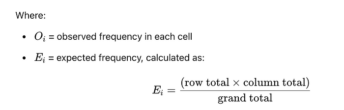
Assumptions

• Expected Frequencies: Each cell’s expected frequency should be at least 5 for the test to be reliable. In a large production dataset, this is likely met.

• Independence: Observations must be independent, reasonable in most machine learning data contexts.

If expected frequencies are too low, Fisher’s Exact Test could be an alternative, but with sufficient data, the Chi-squared Test is standard and effective.

---

Step 1: Sample Dataset

Suppose you have a dataset tracking the categorical variable over time, Using Databricks’ Python environment, I leveraged the scipy.stats library

import pandas as pd
import numpy as np

# Simulated data
data = {
    'Time_Period': ['Older']*1000 + ['Recent']*1000,
    'Payment_Method': (['Credit Card']*400 + ['Debit Card']*400 + [np.nan]*200 +
                       ['Credit Card']*300 + ['Debit Card']*300 + [np.nan]*400)
}
df = pd.DataFrame(data)

# Create a column for missingness status
df['Is_Missing'] = df['Payment_Method'].isna().map({True: 'Missing', False: 'Present'})

Step 2: Create Contingency Table

# Build the contingency table
contingency_table = pd.crosstab(df['Time_Period'], df['Is_Missing'])
print("Contingency Table:")
print(contingency_table)

Output might look like:

Time_Period    Missing  Present  
Older            200      800
Recent           400      600

Step3: Perform the Two-way Chi-squared Test

from scipy.stats import chi2_contingency

# Run the test
chi2, p, dof, expected = chi2_contingency(contingency_table)

print(f"Chi-squared Statistic: {chi2:.4f}")
print(f"P-value: {p:.4f}")
print(f"Degrees of Freedom: {dof}")
print("Expected Frequencies:")
print(expected)

Sample Output:

Chi-squared Statistic: 66.6667
P-value: 0.0000
Degrees of Freedom: 1
Expected Frequencies:
[[300. 700.]
 [300. 700.]]

Interpretation

• Chi-squared Statistic: Measures deviation between observed and expected frequencies.

• P-value: Here, p<0.05p < 0.05p<0.05, so we reject the null hypothesis, indicating a significant association between time period and missingness.

• Conclusion: Missing values are indeed more prevalent in recent data.

Step4: Visualize the Data

import matplotlib.pyplot as plt
import seaborn as sns

sns.heatmap(contingency_table, annot=True, fmt="d", cmap="Blues")
plt.title("Contingency Table: Missing vs. Present by Time Period")
plt.show()

This heatmap visually confirms the increase in missing values in recent data

---

Lessons Learned

This experience reinforced a few key lessons for technical documentation:

• Monitor Data Quality: In production ML, vigilance over input variables is critical. Missing values can silently degrade model performance.

• Choose the Right Tool: The Two-way Chi-squared Test was ideal here, leveraging a contingency table to compare missingness across time. Alternatives like the KS test or Jensen-Shannon distance didn’t align as well with my categorical, binary-framed question.

• Databricks Power: The platform’s ability to handle large-scale data aggregation and integrate with statistical libraries made this analysis seamless.

In the end, we patched the API, retrained the model with cleaner data, and restored our churn predictions to peak accuracy. This little detective story became a staple in our team’s blog, a reminder that even in the high-stakes world of machine learning, the simplest statistical tools can solve the trickiest problems.