Day 9: Logistic Regression – Predicting Yes/No Outcomes
 Saket Khopkar
Imagine you're a marketing analyst, and your job is to predict whether a customer will buy a product or not based on their age and salary. You need a model that gives a clear yes or no answer rather than a continuous number like in linear regression. This is where Logistic Regression comes in!
Today, we'll break it down step by step, making it super simple with real-life examples and a hands-on Python implementation in Jupyter Notebook.
Gentle Definition
Logistic Regression is a classification algorithm used when the target variable is categorical (e.g., Yes/No, Spam/Not Spam, Pass/Fail). Instead of predicting a continuous value like Linear Regression, it predicts probabilities between 0 and 1.
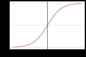
Since we can't use Linear Regression (which predicts continuous values like 2.5 or -1.3), we use the Sigmoid Function to squeeze the predictions between 0 and 1.
The curve you will see for this looks something like this:

The close it is to 1, the more likelihood of the positive results.
✅ If probability > 0.5 → Predict 1 (Yes, the event will happen).
✅ If probability ≤ 0.5 → Predict 0 (No, the event won’t happen).
Examples:
Email Spam Detection: Classifies emails as Spam (1) or Not Spam (0).
Loan Approval System: Predicts whether a loan will be approved (1) or denied (0).
Disease Diagnosis: Determines if a patient has diabetes (1) or does not have diabetes (0).
Predicting Winners: Predicts whether your favourite team will win (1) or lose (0) IPL this season.
Mathematical Explaination
We use Sigmoid function for logistic regressions. The Sigmoid function is given by:

Where:
z = Linear Combinations of Input values [z = w0 + w1×1 + w2×2 + … + wnxn]
e = Euler’s number (≈2.718)
This function evalueates and ensures that if:
If z is large (positive), σ(z) is close to 1 (event likely to happen).
If z is small (negative), σ(z) is close to 0 (event unlikely to happen).
If z=0, the probability is exactly 0.5 (uncertain).
This helps us convert predictions into probabilities between 0 and 1, making it useful for classification.
Preety easy right? Well we haven’t seen the coding way yet…
Simple Example Discussion
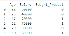
Suppose a company wants to predict a customer will buy their product or not based on the below data:
| Age | Salary | Bought (Yes = 1 ; No = 0) |
| 22 | 30000 | 0 |
| 25 | 40000 | 0 |
| 47 | 70000 | 1 |
| 52 | 75000 | 1 |
| 29 | 50000 | 0 |
| 50 | 65000 | 1 |
So you have a clearer picture ahead of you.
We will be using this same example for code level next.
Code Time
For this demonstartion we will follow the exact same path as in previous blogs.
import numpy as np
import pandas as pd
import matplotlib.pyplot as plt
import seaborn as sns
from sklearn.model_selection import train_test_split
from sklearn.preprocessing import StandardScaler
from sklearn.linear_model import LogisticRegression
from sklearn.metrics import accuracy_score, confusion_matrix, classification_report

# Sample dataset
data = {'Age': [22, 25, 47, 52, 29, 50],
        'Salary': [30000, 40000, 70000, 75000, 50000, 65000],
        'Bought_Product': [0, 0, 1, 1, 0, 1]}

df = pd.DataFrame(data)
print(df)

# Features (X) and Target (Y)
X = df[['Age', 'Salary']]
y = df['Bought_Product']

# Split data into training (80%) and testing (20%)
X_train, X_test, y_train, y_test = train_test_split(X, y, test_size=0.2, random_state=42)

print(f"Training samples: {len(X_train)}, Testing samples: {len(X_test)}")

# Feature Scaling - Since age and salary are on different scales, we use StandardScaler to normalize them.
scaler = StandardScaler()
X_train = scaler.fit_transform(X_train)
X_test = scaler.transform(X_test)

# Train the model
model = LogisticRegression()
model.fit(X_train, y_train)

# Predict on test set
y_pred = model.predict(X_test)
print("Predicted values:", y_pred)
# Accuracy Score
accuracy = accuracy_score(y_test, y_pred)
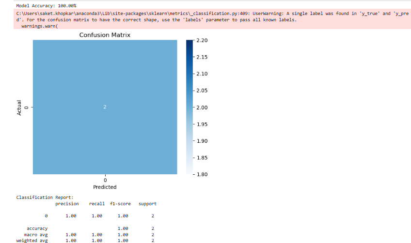
print(f"Model Accuracy: {accuracy * 100:.2f}%")

# Confusion Matrix
conf_matrix = confusion_matrix(y_test, y_pred)
sns.heatmap(conf_matrix, annot=True, cmap="Blues", fmt='d')
plt.xlabel('Predicted')
plt.ylabel('Actual')
plt.title('Confusion Matrix')
plt.show()

# Classification Report
print("Classification Report:\n", classification_report(y_test, y_pred))

The job of confusion matrix is to show the number of correct and incorrect predictions. Accuracy Score is used to evaluate how well our model performs, for our case, its 100% accurate. The fields Precision, Recall and F1 Score evaluate classifcation performance.
Well this is all about Logistic Regression. A sigmoid curve, predicting values between 0 and 1 and more the closer to 1, the more chances the result will be positive.
Logistic Regression is great for binary classification (Yes/No, 1/0). In our code, we evaluated the model with accuracy, confusion matrix, and classification report.
Again, its my duty to remind fellow learners that tweak with the data, the more you play with it, the more variations you may notice. This helps learning better. I know this is becomming a repaeated lines, but if you are following up Day wise series, it would be beneficial.
For now, Ciao!
Subscribe to my newsletter
Read articles from Saket Khopkar directly inside your inbox. Subscribe to the newsletter, and don't miss out.
Written by

Saket Khopkar
Saket Khopkar
Developer based in India. Passionate learner and blogger. All blogs are basically Notes of Tech Learning Journey.