Efficient Methods for Generating Zonal Statistics in GIS

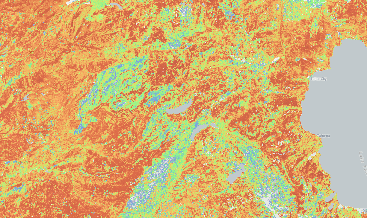
Zonal Statistics is the name we give to metrics extracted from rasters (rasters in the GIS world are images/matrixes), given a particular area.

These metrics can be extracted for the entire raster dataset or subset according to a particular polygon. The most common metrics extracted in zonal statistics processes are minimum, maximum, average, and standard deviation.

These particular numbers are used in different contexts but are instrumental to extract a generalized representation of a specific phenomenon inside that area. In the picture above, the full raster represents probability of high severity fire (this dataset comes from California’s Regional Resource Kits). Using the polygons above, we can understand the average probability for a particular region.

These numbers can then be fed into data models. Scientists use several computational models to simulate the real world, such as how a fire spreads in a given landscape or how much damage a particular fire will cause.

We are working with large rasters and feeding these numbers into ForSys, a valuable landscape planning model for understanding optimized areas for treatments/interventions. ForSys inputs are matrixes of numbers, with several phenomenons represented, and its outputs are priority areas for intervention (you also have to tell ForSys how to prioritize each phenomenon and particular restrictions).

Planscape

Planscape is a tool that allows landscape planners to create, manage, and simulate several different scenarios, using ForSys, in a very convenient web interface. Planscape right now targets the state of California and works in three different resolutions:

Large (500 acres per polygon)
Medium (200 acres per polygon)
Small (10 acres per polygon)

Over 24 million of these polygons cover California, and they are used to extract Zonal Statistics from over 200 different datasets. Each dataset is composed of rasters of 30m pixels. This means that we have to crunch a lot of numbers before sending this information to our optimization layer, ForSys.

Since we have a lot to do, the speed of calculating Zonal statistics is essential.

Rules of the Game

Our rules to run this benchmark were straightforward:

Same machine in all trials (i7, 16Gb RAM, no GPU laptop)
5 runs per method
PostgreSQL 16, PostGIS 3.5.2
Python 3.12
Local IO (no network calls)
One raster with 30 meter resolution

It’s hard to extract precise timings because some of the methods are very different, leading to different considerations, but the idea is to be directionally correct.

Methods

PostGIS - with rasters stored in the database
PostGIS - with rasters stored in disk
Rasterstats - Original code
Rasterstats - Custom Code #1
Rasterstats - Custom Code #2

PostGIS

Planscape uses PostGIS, so it was our first idea. It is widely available, easy to use, and allows us to prototype the algorithm quickly.

The code we used to generate the zonal statistics is pretty much the same, between both versions, in and out of database rasters:

WITH stand AS (
      SELECT
        id,
        ST_Transform(ss.geometry, 3857) AS geometry
      FROM stands_stand ss
      WHERE
        id = p_stand_id
    ),

    stats AS (
      SELECT
        (ST_SummaryStats(ST_Clip(cc.rast, s.geometry))).*
      FROM high_sev_fire cc, stand s
      WHERE
        s.geometry && cc.rast AND
        ST_Intersects(s.geometry, cc.rast)
    )

    SELECT 
      p_stand_id,
      min(ss.min) AS min,
      max(ss.max) AS max,
      sum(ss.mean * ss.count)/sum(ss.count) AS avg,
      sum(ss.sum) AS sum,
      sum(ss.count) AS count
    FROM
      stats ss

When we executed this we were able to obtain the following numbers:

In Database: 282 polygons per second
Out of Database: 137 polyhons per second

These numbers are not really good.

Rasterstats

Rasterstats is a Python package based on the fantastic rasterio. Rasterstats is pretty fast and uses Numpy under the hood.

from rasterstats import zonal_stats
raster_file = "data/raster.tif"
geojson = "data/stands.geojson"
stats = "min max count mean sum"
out = list(zonal_stats(geojson, raster_file, stats=stats, geojson_out=True))

The code is straightforward and does not have a lot of secrets. One particular important thing here is to notice that the raster is also using the EPSG:4326 projection.

587 polygons per second

Rasterstats - Custom Code #1

We’ve made some assumptions about rasterstats code that we considered we could make it faster.

We took the primary zonal_stats function and stripped out everything that did not make sense for our use case. This function can be seen in our repository.

def get_zonal_stats(
    geom,
    raster,
    band=1,
    nodata=None,
    affine=None,
    all_touched=False,
    boundless=True,
    **kwargs,
):
    """Custom zonal statistics function. Strips out everything we don't
    need from the original one.
    """

    with Raster(raster, affine, nodata, band) as rast:
        geom_bounds = tuple(geom.bounds)
        fsrc = rast.read(bounds=geom_bounds, boundless=boundless)

        rv_array = rasterize_geom(geom, like=fsrc, all_touched=all_touched)

        # nodata mask
        isnodata = fsrc.array == fsrc.nodata

        # add nan mask (if necessary)
        has_nan = np.issubdtype(fsrc.array.dtype, np.floating) and np.isnan(
            fsrc.array.min()
        )
        if has_nan:
            isnodata = isnodata | np.isnan(fsrc.array)

        # Mask the source data array
        # mask everything that is not a valid value or not within our geom
        masked = np.ma.MaskedArray(fsrc.array, mask=(isnodata | ~rv_array))

        if sys.maxsize > 2**32 and issubclass(masked.dtype.type, np.integer):
            accum_dtype = "int64"
        else:
            accum_dtype = None  #

        if masked.compressed().size == 0:
            # nothing here, fill with None and move on
            return {
                "min": None,
                "max": None,
                "mean": None,
                "count": 0,
                "sum": None,
            }
        return {
            "min": float(masked.min()),
            "max": float(masked.max()),
            "mean": float(masked.mean(dtype=accum_dtype)),
            "count": int(masked.count()),
            "sum": float(masked.sum(dtype=accum_dtype)),
        }

The calling function:

# projected is a GeoJSON datastructure with several features
projected = {"type": "FeatureCollection", "features": []}  
raster_file = "path/to/raster.tif"
def _zonal_stats(g):
    return get_zonal_stats(g, raster_file)
custom_out = list(map(_zonal_stats, projected))

In this particular case, we are letting rasterstats open the raster.

The result was disappointing:

137 polygons per second

Rasterstats - Custom Code #2

Why was our first try slower? We opened our dataset and fed it to raster stats incorrectly, leading to a lot of overhead while opening raster files.

In the second attempt, we tweaked the client code that called our custom function:

src = rasterio.open(raster_file)
affine = rasterio.transform.guard_transform(src.transform)
array = src.read(1)
def _zonal_stats_opened(g):
    return get_zonal_stats(g, array, affine=affine)
custom_out_already_open = list(map(_zonal_stats_opened, projected))

The main difference here is that we:

Opened the dataset ourselves
Computed the affine transformation, outside of our hot path
Read the raster data only once. The previous function would read only a subset of the array, but it is still relatively slow.

As it turns out, IO is quite expensive. Our results:

729 polygons per second

Takeaways

This work enabled us to move from a pre-computed statistics model to obtaining the statistics during runtime, which allows us to use new datasets in Planscape. This is a significant win, enabling Planscape to be used in the entire Continental United States and the rest of the world.
The best results might not be the most complex ones. rasterstats is incredibly efficient by itself. We are not using our custom function in Planscape, but we are opening the datasets only once, like in this benchmark.
Do one change at a time and measure!