Demystifying Compiler Design: Syntax, Semantics, and Runtime Explained
 Aakashi Jaiswal
What is a Compiler?
A compiler is a specialized translator program that reads a program written in a high-level source language and translates it into a target language, often machine or assembly language. The compilation process involves several phases, each transforming the source program from one representation to another. These phases are broadly categorized into:
Analysis phase: Includes lexical analysis, syntax analysis, and semantic analysis.
Synthesis phase: Includes intermediate code generation, code optimization, and target code generation.
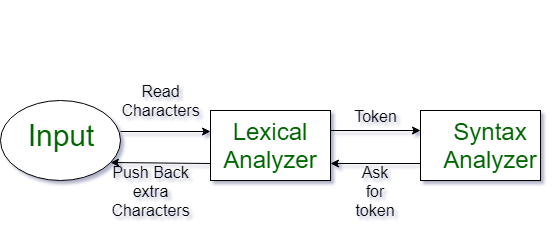
Lexical analysis is the very first phase of the compiler and is crucial for the subsequent phases to work correctly.
Lexical Analysis: Definition and Purpose
Lexical Analysis (also called scanning) is the process of converting a sequence of characters in the source code into a sequence of tokens. It reads the input source code character by character and groups these characters into meaningful sequences called lexemes, which correspond to tokens.
The lexical analyzer serves several key functions:
Tokenization: Breaking the input stream into tokens such as keywords, identifiers, constants, operators, and punctuation symbols.
Removing whitespace and comments: These are ignored as they do not affect the program semantics.
Error detection: Identifying invalid tokens or illegal character sequences and reporting lexical errors.
Interface with the parser: Providing tokens to the syntax analyzer (parser) on demand.
For example, in the C statement int value = 100;, the lexical analyzer identifies the tokens: int (keyword), value (identifier), = (operator), 100 (constant), and ; (symbol).
Tokens and Lexemes
Lexeme: A sequence of characters in the source program that matches the pattern for a token.
Token: A category or class of lexemes. Tokens are defined by patterns, usually described using regular expressions.
Typical tokens include:
Keywords (e.g.,
int,return)Identifiers (variable names)
Constants (numeric or string literals)
Operators (e.g.,
+,=)Punctuation symbols (e.g.,
;,{,})
The lexical analyzer uses predefined grammar rules and regular expressions to recognize these tokens.
How Lexical Analysis Works
Input: The source code is fed as a stream of characters.
Scanning: The lexical analyzer scans the input character stream, eliminating whitespace and comments.
Pattern Matching: It matches sequences of characters against token patterns using regular expressions.
Token Generation: Once a lexeme matches a token pattern, the token is generated and passed to the parser.
Error Handling: If no valid token is found for a lexeme, a lexical error is reported.
The parser requests tokens from the lexical analyzer one at a time, which means the lexical analyzer produces tokens on demand.
Architecture of Lexical Analyzer
Input Buffer: Holds the source code characters.
Scanner: Reads characters and groups them into lexemes.
Token Generator: Converts lexemes into tokens.
Symbol Table: Stores information about identifiers and constants.
Error Handler: Detects and reports lexical errors.
The lexical analyzer often uses finite automata generated from regular expressions to efficiently recognize tokens.
Roles and Responsibilities of Lexical Analyzer
Remove unnecessary characters like white spaces, tabs, and comments.
Read the source code character by character.
Identify tokens and pass them to the syntax analyzer.
Maintain and update the symbol table with identifiers.
Detect lexical errors and provide meaningful error messages with source location.
Facilitate smooth parsing by providing a clean token stream.
Advantages of Lexical Analysis
Simplifies parsing by reducing the complexity of input.
Helps in error detection early in the compilation process.
Improves efficiency by eliminating irrelevant characters.
Supports modular compiler design by separating concerns.
Summary
Lexical analysis is the first and foundational phase of a compiler.
It transforms raw source code into tokens by scanning and pattern matching.
Tokens include keywords, identifiers, constants, operators, and symbols.
It removes whitespace and comments, detects errors, and interfaces with the parser.
Lexical analyzers are implemented using regular expressions and finite automata.
This phase is essential for the correctness and efficiency of the entire compilation process.
This comprehensive understanding of lexical analysis lays the groundwork for deeper studies into syntax analysis and other compiler phases.
Parsing is a fundamental process in computer science, especially in compiler design, where it involves analyzing a sequence of symbols (tokens) to determine its grammatical structure according to a given formal grammar. The goal of parsing is to build a structural representation of the input, such as a parse tree or abstract syntax tree, while checking for syntactical correctness.
Parsing and Parsers
A parser is a software component that takes input data-usually text or code-and organizes it into a hierarchical structure based on grammar rules. It typically follows lexical analysis, where the input is divided into tokens.
Parsers can be hand-written or generated by parser generators. They are widely used in compilers, interpreters, data processing, and natural language processing.
Types of Parsing
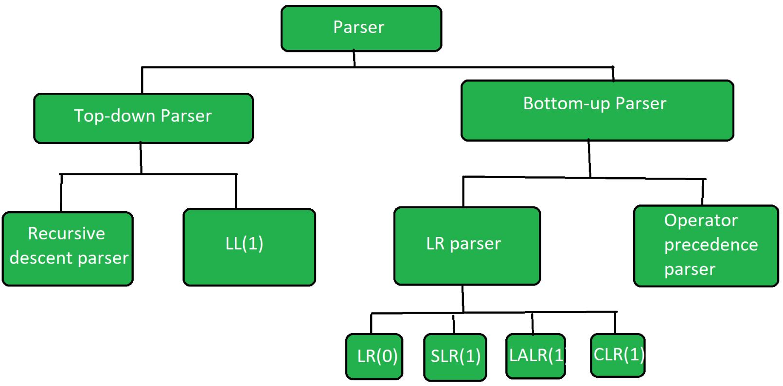
Parsing methods are broadly classified into two categories based on how they analyze the input and derive the parse tree:
1. Top-Down Parsing
Concept: Starts from the start symbol of the grammar and tries to rewrite it to the input string by applying production rules, expanding non-terminals to match the input tokens.
Process: Attempts to find a leftmost derivation of the input by recursively expanding grammar rules from the top (start symbol) down to terminals.
Example Techniques:
Recursive Descent Parsing: Implements the grammar as a set of recursive procedures, each corresponding to a non-terminal. It reads input left to right and constructs the parse tree top-down.
Predictive Parsing (LL Parsing): A form of top-down parsing that uses lookahead tokens to decide which production to use without backtracking.
Limitations: Cannot handle left-recursive grammars directly and may require grammar transformations.
Derivation Type: Produces leftmost derivations.
2. Bottom-Up Parsing
Concept: Starts from the input tokens and attempts to reconstruct the start symbol by reducing substrings (handles) into non-terminals, effectively building the parse tree from leaves (tokens) up to the root (start symbol).
Process: Finds the rightmost derivation of the input in reverse.
Example Techniques:
Shift-Reduce Parsing: Uses a stack to shift input tokens and reduce sequences on the stack to non-terminals based on grammar rules.
LR Parsing: A powerful bottom-up parsing method that reads input left to right and produces a rightmost derivation in reverse.
Derivation Type: Produces rightmost derivations (in reverse).
Shift-Reduce Parsing Explained
Shift-reduce parsing is a common bottom-up parsing technique characterized by two main operations:
Shift: Move the next input token onto the parsing stack.
Reduce: When the top of the stack matches the right-hand side of a grammar production, replace it with the corresponding left-hand side non-terminal.
The parser alternates between these steps to gradually reduce the input string to the start symbol. This method is efficient and forms the basis of many LR parsers.
FIRST and FOLLOW Functions
These functions are essential in constructing parsing tables for predictive (top-down) parsers, helping the parser decide which production rule to apply.
FIRST Function
Definition: For a grammar symbol or string of symbols α\alphaα, FIRST(α\alphaα) is the set of terminals that can appear at the beginning of any string derived from α\alphaα.
Purpose: Helps determine which production to use when the parser encounters a particular input token.
Computation Rules:
If α\alphaα is a terminal, FIRST(α\alphaα) is just {α}\{ \alpha \}{α}.
If α\alphaα is a non-terminal, FIRST(α\alphaα) includes the FIRST sets of its productions.
If a production can derive the empty string ϵ\epsilonϵ, then ϵ\epsilonϵ is included in FIRST(α\alphaα).
For a string Y1Y2…YnY_1 Y_2 \ldots Y_nY1Y2…Yn, FIRST is computed by checking FIRST(Y1Y_1Y1), and if it contains ϵ\epsilonϵ, then FIRST(Y2Y_2Y2) is also considered, and so on.
FOLLOW Function
Definition: For a non-terminal NNN, FOLLOW(NNN) is the set of terminals that can appear immediately to the right of NNN in some "sentential" form derived from the start symbol.
Purpose: Used to decide when to apply productions that can derive ϵ\epsilonϵ and for constructing parsing tables.
Computation Rules:
The end-of-input marker (often $) is in FOLLOW of the start symbol.
For a production A→αBβA \to \alpha B \betaA→αBβ, everything in FIRST(β\betaβ) except ϵ\epsilonϵ is in FOLLOW(BBB).
If β\betaβ can derive ϵ\epsilonϵ, then FOLLOW(AAA) is also in FOLLOW(BBB).
Summary of Parsing Concepts
| Aspect | Description |
| Parsing | Analyzing input tokens to build a syntax tree based on grammar rules. |
| Parser | Software that performs parsing, often after lexical analysis. |
| Top-Down Parsing | Starts from the start symbol, expands productions to match input; leftmost derivation. |
| Bottom-Up Parsing | Starts from input tokens, reduces to start symbol; rightmost derivation in reverse. |
| Shift-Reduce Parsing | Bottom-up technique using shift and reduce operations on a stack to parse input. |
| FIRST Function | Set of terminals that begin strings derived from a grammar symbol or string. |
| FOLLOW Function | Set of terminals that can appear immediately after a non-terminal in some derivation. |
Parsing is a core step in compiler design and many other areas where structured input needs to be analyzed and understood. The choice of parsing technique depends on the grammar and the requirements of the application.
Syntax Directed Translation (SDT)
Syntax Directed Translation is a method used in compiler design where the translation of a source program is guided by its syntax, specifically by the context-free grammar of the language. It integrates semantic analysis with parsing by associating semantic rules or actions with the grammar productions.
Core Concept: Each production in a context-free grammar is augmented with semantic rules (also called semantic actions) that specify how to compute attributes related to the grammar symbols. These attributes carry semantic information such as types, values, or code fragments.
Attributes: Attributes are pieces of information attached to grammar symbols (terminals and non-terminals). They can represent various data like types, values, memory locations, or code snippets. Attributes are classified into:
Synthesized Attributes: Computed from the attributes of child nodes in the parse tree.
Inherited Attributes: Passed down from parent or sibling nodes.
Semantic Actions: These are snippets of code or instructions executed at specific points during parsing. They can compute attribute values, generate intermediate code, or update symbol tables. Semantic actions are embedded in grammar productions, typically enclosed in braces
{}.Parsing and Semantic Actions:
In Top-Down Parsing, semantic actions are executed when a production is expanded.
In Bottom-Up Parsing, semantic actions are executed when a production is reduced.
Purpose: SDT allows the compiler to perform semantic analysis and generate intermediate code directly during parsing, making the compilation process more efficient and structured.
Example: For an expression grammar, semantic actions can compute the value of expressions or produce intermediate code for arithmetic operations by combining the attributes of subexpressions.
Type Checking
Type checking is a critical phase of semantic analysis in a compiler that ensures the program adheres to the language's type rules. It verifies that operations in the program are semantically correct with respect to data types.
Type System: Defines the rules for how types interact in a language. For example, ensuring operands of arithmetic operations are numeric or that function calls have correct argument types.
Static Type Checking: Performed at compile time to catch type errors before program execution. It helps in detecting errors like applying arithmetic on incompatible types or passing incorrect arguments to functions.
Dynamic Type Checking: Performed at runtime, less common in statically typed languages.
Tasks in Type Checking:
Verify operand types for operators (e.g.,
modoperator requires integer operands).Check array indexing uses an integer index on an array type.
Ensure functions are called with the correct number and types of arguments.
Determine types of expressions and propagate type information through the parse tree.
Type Conversion: Sometimes implicit or explicit conversions are needed to make operands compatible (e.g., converting integer to float).
Symbol Tables
Symbol tables are data structures used by compilers to store information about identifiers (variables, functions, constants, etc.) encountered in the source program.

Contents of Symbol Table:
Lexeme (the actual name of the identifier)
Token type (identifier, keyword, operator, etc.)
Semantic information (data type, scope level, memory location, etc.)
Additional attributes like number of parameters for functions, return types, etc.
Role in Compilation:
During lexical analysis, user-defined identifiers and literals are entered into the symbol table.
The parser uses the symbol table to retrieve token information.
Semantic analysis uses the symbol table to check types and scopes.
Intermediate code generation may use symbol table information for memory allocation.
Scope Management:
Symbol tables support nested scopes by maintaining a stack of tables or using linked structures.
When entering a new scope (like a procedure or block), a new symbol table is created and pushed onto the stack.
When exiting the scope, the symbol table is popped.
This allows correct resolution of identifiers according to their scope.
Building Symbol Tables:
Can be done during parsing by embedding semantic actions that insert identifiers into the symbol table.
Alternatively, the Abstract Syntax Tree (AST) can be built first, then traversed to populate the symbol table and perform type checking.
Integration of Syntax Directed Translation, Type Checking, and Symbol Tables
Syntax Directed Translation schemes embed semantic actions in grammar productions to perform tasks like building symbol tables and type checking during parsing.
Attributes computed during SDT include type information, which is stored and referenced in the symbol table.
Type checking rules are enforced by semantic actions that consult the symbol table to verify types and scopes.
This integration ensures that semantic errors are caught early and that intermediate code generation has accurate semantic information.
Type Equivalence
Type equivalence defines when two types are considered the same during type checking. It is essential for verifying assignments, parameter passing, and operations involving multiple types.
Structural Equivalence
Definition: Two types are structurally equivalent if they have the same structure or composition, regardless of their names.
How it works: The compiler compares the components of the types recursively. For example, two arrays of integers with the same size are structurally equivalent, even if they have different type names.
Example:
  texttype A = array[1..10] of integer;
  type B = array[1..10] of integer;
Here,
AandBare structurally equivalent because both are arrays of 10 integers.
Name Equivalence
Definition: Two types are name equivalent if they have the same type name or originate from the same type declaration.
How it works: The compiler treats types as equivalent only if they share the exact same name, even if their structures are identical.
Example:
  texttype A = array[1..10] of integer;
  type B = array[1..10] of integer;
Here,
AandBare not name equivalent because they are declared as distinct types, despite having the same structure.
Type Conversion
Type conversion is the process of converting a value from one data type to another. It ensures that operations involving different types can be performed correctly.
Implicit Conversion (Coercion)
Definition: Automatic conversion performed by the compiler without programmer intervention.
When it happens: When an expression involves different types, the compiler converts one type to another to make the operation valid.
Example: Assigning an integer to a float variable automatically converts the integer to a float.
Note: Implicit conversions can sometimes lead to subtle bugs or loss of precision.
Explicit Conversion (Casting)
Definition: Conversion explicitly requested by the programmer.
How it works: The programmer uses a cast operator to specify the target type.
Example:
cfloat x = (float) 10; // Explicitly converts integer 10 to floatUse case: Used when implicit conversion is not available or when the programmer wants to override default conversion rules.
Runtime Environment Management in compiler design is a crucial aspect that deals with how a program is executed on a target machine after being compiled. It involves managing the state of the machine, memory allocation, procedure calls, variable storage, and interaction with system resources to ensure smooth execution of the program.
What is Runtime Environment?
The runtime environment refers to the state of the target machine during the execution of a program. It includes various components such as:
Software libraries
Environment variables
Memory resources
Runtime support systems
This environment provides the necessary services to the processes running the program, such as memory management and communication between the program and the operating system. The runtime environment is distinct from the compile-time environment and is concerned with the actual execution of the program instructions on the machine.
Role of Runtime Support System
The runtime support system is a package usually generated along with the executable program. It acts as an intermediary between the running process and the runtime environment, handling:
Memory allocation and deallocation during program execution
Procedure call management
Parameter passing
Process communication
It ensures that the program runs efficiently by managing resources dynamically as the program executes.
Key Concepts in Runtime Environment Management
1. Program Execution and Activation Tree
When a program runs, it executes a sequence of instructions that may involve calling procedures or functions. The runtime environment manages this flow of control, which can be represented as an activation tree. Each node in the tree corresponds to an activation record (or stack frame) representing a procedure call and its execution state.
2. Memory Management
Memory management in the runtime environment involves allocating space for different entities:
Code (Text Segment): The compiled program instructions, which are static and known at compile time.
Procedures: Their code is static, but calls to them are dynamic and managed using a stack structure to handle nested calls and returns.
Variables: Variables may be global, local, or dynamically allocated. Local variables and procedure parameters are typically stored on the stack, while dynamically allocated variables use the heap.
3. Storage Allocation Schemes
There are three primary storage allocation schemes managed by the runtime environment:
Static Allocation: Memory locations are fixed at compile time and do not change during execution. This is used for global variables and constants.
Stack Allocation: Used for procedure calls and local variables. The stack grows and shrinks dynamically with procedure activations and returns.
Heap Allocation: Used for dynamic memory allocation where variables are created and destroyed at runtime, such as objects or data structures.
4. Parameter Passing
The runtime environment handles the mechanism of passing parameters to procedures, which can be done by value, by reference, or other methods depending on the language semantics. This is managed through the activation records and calling conventions defined by the runtime system.
Interaction with Operating System
The runtime environment often acts as an abstraction layer over the operating system, managing system calls and resources such as file I/O, networking, and threading. It hides the complexity of different operating system interfaces and provides a consistent execution environment for the program.
Advanced Features
Some runtime environments provide additional features such as:
Garbage collection to automatically manage memory
Just-In-Time (JIT) compilation to optimize code at runtime
Support for parallel execution and synchronization primitives
Debugging and error handling mechanisms
Summary
Runtime Environment Management in compiler design encompasses all the mechanisms and structures that support the execution of a compiled program on a target machine. It involves:
Providing an execution state that includes libraries, variables, and memory
Managing procedure calls and control flow through activation records and the activation tree
Allocating and deallocating memory dynamically using stack and heap
Handling parameter passing and interfacing with the operating system
Supporting advanced runtime features for efficient and safe program execution
What is an Activation Record?
An activation record (also called a stack frame) is a data structure that contains all the information needed to manage a single execution of a procedure or function. This includes parameters, local variables, return addresses, saved registers, and bookkeeping information.
Location for Activation Record
Where activation records (ARs) — the data structures storing info about function calls — are placed depends on the language:
1. Static Area:
Used in early languages like FORTRAN.
Memory is fixed at compile time.
Parameters are copied in/out when a procedure is invoked.
No recursion possible (only one activation per procedure).
2. Stack Area:
Used in languages like C, Pascal, Java.
Each function call pushes an activation record on the stack.
Function return pops the record.
Works well for non-recursive, non-returned local variables.
3. Heap Area:
Used in functional languages like LISP.
Required when functions are first-class citizens (i.e., they can be returned from other functions).
Processor Registers
Used during execution:
Program Counter (PC): points to the next instruction.
Stack Pointer (SP): top of the call stack.
Frame Pointer (FP): base of the current activation record.
Argument Pointer (AP): region in AR for function parameters.
Environment Types
Without Local Procedures (e.g., C):
All functions are global.
Frame pointer allows accessing current locals.
Dynamic link (control link): stored in AR; points to previous AR on stack.
With Local Procedures (e.g., Pascal):
Procedures can be nested.
Access link is added to AR to reach non-local variable declarations.
Compiler generates code to traverse
daccess links to reach required environment.
Accessing Variables
Variables are accessed using offsets from the frame pointer.
Example:
- For function
g(m)with localy, offset ofmis+4(fp)andyis-6(fp).
- For function
Activation Record Creation and Deletion
🔹 Phase 1: Function Call – Caller Setup
This is what happens when one function calls another:
The caller prepares everything the callee needs:
Allocates a space (activation record) for the callee.
Stores the function’s arguments (parameters).
Saves the return address (to resume after callee finishes).
Saves necessary register values.
Updates the frame pointer to point to the callee’s frame.
Jumps to the start of the callee’s code.
🔹 Phase 2: Function Call – Callee Setup
Now the called function (callee) takes over:
It saves its own CPU state (registers).
Allocates space for local variables inside its activation record.
Initializes those local variables (if needed).
Execution of the function body begins.
🔹 Phase 3: Function Return – Cleanup
Once the callee finishes its task, this is what happens:
The callee:
Stores the return value.
Restores any registers it changed.
Frees local memory space.
Restores the previous frame pointer.
Jumps back to the caller using the saved return address.
The caller resumes:
Retrieves the return value.
Cleans up the callee’s activation record.
Restores its saved registers and continues executing.
Memory View of Activation Record
| Field | Purpose |
| Return address | Resume point in caller |
| Control link | Frame pointer to caller’s AR |
| Access link | (If needed) link to outer scope AR |
| Local variables | Function-local variables |
| Temporaries | Temporary results |
| Parameters | Passed by caller |
| Saved registers | Any saved CPU registers |
Translation Rules (for control flow)
Case/Switch Statement Translation
Function Calls (Calling & Return Sequences)
Function Code Generation Strategies
1️⃣ Translation Rules for Control Flow
These rules guide how to generate intermediate code (typically three-address code) for control-flow statements like if, if-else, while, etc.
Rule 1: If Statement
Grammar: S → if B then M S1
Action:
backpatch(B.truelist, M.quad)
S.nextlist = merge(B.falselist, S1.nextlist)
🧠 Explanation:
B.truelist contains jumps that must go to the “then” part (S1).
M.quad is the line number (or nextquad()) where S1 begins.
B.falselist holds jumps when the condition fails — merged with any jumps coming after S1.
Rule 2: If-Else Statement
S → if B then M1 S1 N else M2 S2
Action:
backpatch(B.truelist, M1.quad)
backpatch(B.falselist, M2.quad)
S.nextlist = merge(S1.nextlist, N.nextlist, S2.nextlist)
🧠 Explanation:
Two entry points: S1 (then) and S2 (else).
N creates an unconditional jump to skip “else” after executing “then”.
All exits (nextlist) from both branches are merged.
Rule 3: While Loop
S → while M1 B do M2 S1
Action:
backpatch(S1.nextlist, M1.quad) // Jump back to recheck loop
backpatch(B.truelist, M2.quad) // Proceed to loop body
S.nextlist = B.falselist // Exit condition
emit('goto' M1.quad) // Jump back to condition
🧠 Explanation:
Repeats loop until B is false.
Jump from end of body back to the condition.
On false, jump to code after loop.
Rule 4: begin...end Block
S → begin L end
S.nextlist = L.nextlist
L → L1 M S
backpatch(L1.nextlist, M.quad)
L.nextlist = S.nextlist
L → S
L.nextlist = S.nextlist
🧠 Explanation:
Allows compound statements (block with multiple sub-statements).
Backpatching ensures correct order of statements.
Rule 5: Epsilon Nonterminals
M → ε
M.quad = nextquad()
N → ε
N.nextlist = nextquad()
emit(‘goto ...’)
🧠 Explanation:
These help reserve jump locations for control transfers.
Backpatch later when true targets are known.
2️⃣ Example Code Generation
For:
    begin
      while a > b do
      begin
        x = y + z;
        a = a - b;
      end
      x = y - z;
    end
Three-address code:
    1: if a > b goto 3
    2: goto 8
    3: t1 = y + z
    4: x = t1
    5: t2 = a - b
    6: a = t2
    7: goto 1
    8: x = t3
🧠 Explanation:
Line 1 checks loop condition.
Line 2 jumps to after loop if false.
Lines 3–6 are loop body.
Line 7 restarts the loop.
Line 8 continues after loop.
3️⃣ Case / Switch Statement Translation
General Format:
    switch(E) {
      case c1: ...
      case c2: ...
      ...
      default: ...
    }
Implementation Approaches:
Linear Search
Compare one by one.
Cheap when few cases.
Binary Search
- Faster for larger sorted case sets.
Jump Table (most efficient for dense case values)
Compute:
if E < cmin → default
if E > cmax → default
else: jump to JumpTable[E]
JumpTable maps values directly to addresses.
🧠 Summary:
Dense values ⇒ Jump Table.
Sparse values ⇒ Linear or Binary Search.
4️⃣ Function Calls
Function call handling is split into two phases:
🔷 Calling Sequence
Caller’s Responsibilities:
Evaluate arguments
Use param instructions to pass them Example: param t
Save return address and current state
Emit: call f, n (n = number of arguments)
Callee’s Responsibilities:
Save its own registers
Set up activation record
Allocate memory for locals
Emit: enter m (m = space needed)
🔶 Return Sequence
Callee’s Responsibilities:
Place return value
Reset stack and frame pointers
Emit: return x
Caller’s Responsibilities:
Retrieve returned value
Emit: retrieve x
Example Code for a Call
X = f(0, y + 1) – 1
Three-address code:
    t1 = y + 1
    param t1
    param 0
    call f, 2
    retrieve t2
    t3 = t2 – 1
    x = t3
🧠 Each param is pushed before the call; value is retrieved and used.
5️⃣ Function Code Generation Strategies
Problem: How do you emit enter m when you don’t know m at the start?
Two Solutions:
A. Generating Final Code in a List
Generate code in a temporary list
Backpatch enter m once function size is known
Pro: More optimization options
Con: Slower, uses more memory
B. Using Pair of Goto Statements
emit goto labelX
emit function body
backpatch labelX with real enter m
Tricky but avoids holding function body in memory
Summary Table
| Topic | Key Concepts |
| Control Flow Translation | Uses backpatching, true/false lists, merge |
| Loop Handling | While loops jump back to condition check |
| Switch-case Implementation | Linear search, binary search, jump table |
| Function Calls | Split into calling and return sequences |
| Code Generation Techniques | Use backpatching or placeholder gotos |
Subscribe to my newsletter
Read articles from Aakashi Jaiswal directly inside your inbox. Subscribe to the newsletter, and don't miss out.
Written by
Aakashi Jaiswal
Aakashi Jaiswal
Coder | Winter of Blockchain 2024❄️ | Web-Developer | App-Developer | UI/UX | DSA | GSSoc 2024| Freelancer | Building a Startup | Helping People learn Technology | Dancer | MERN stack developer