Introduction: Neural networks have come a long way from the simple perceptron to massive transformer models. At their core, however, both are built on the same concept: parameters (weights) that are learned through training. In this post, we’ll start with a single perceptron — examining its inputs, weights, and activation — then show how the same principles scale up to modern large language models (LLMs) like GPT-3. Along the way, we’ll include code snippets and diagrams to bridge intuition from one neuron to billions.

Understanding a Single Perceptron

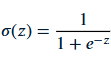
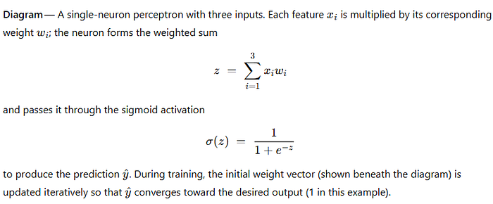
A perceptron is the simplest neural network — essentially one neuron. It takes several inputs, each associated with a weight, computes a weighted sum, and passes that sum through an activation function (historically a step function or sigmoid) to produce an output.

If we include a bias term, the formula for a perceptron’s output y given inputs x1,…,xn is:

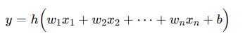
Where wi are the weights, b is the bias, and h() is the activation function such as a sigmoid

How does a perceptron “learn”?

Learning means finding the right weights (and bias) such that the perceptron produces the desired output for given inputs. We start with random weight values and then adjust them iteratively using training examples. The perceptron training algorithm (for a continuous activation like sigmoid) typically works as follows:

• Initialize weights to small random numbers (e.g., between -1 and 1).

• For each training example, compute the output with current weights.

• Compare the output to the expected output (ground truth) to calculate an error.

• Use the error to adjust the weights in the direction that reduces the error (this is often done via gradient descent on the error with respect to each weight).

This process of adjusting weights based on error is repeated for many iterations (epochs) until the error is minimized.

Perceptron in Code

Let’s illustrate a perceptron with a simple Python class called SimpleNeuralNet. This class implements a single-layer neural network with one neuron (a perceptron) that can be trained on examples. It uses a sigmoid activation function for learning a continuous output.

import numpy as np

class SimpleNeuralNet:
    def __init__(self):
        np.random.seed(1)  # for reproducibility
        # Initialize weights for 3 inputs (3x1 vector) with values in [-1, 1)
        self.weight_matrix = 2 * np.random.random((3, 1)) - 1

    def _sigmoid(self, x):
        return 1 / (1 + np.exp(-x))

    def _sigmoid_derivative(self, x):
        # derivative of sigmoid (assuming x has already been passed through sigmoid)
        return x * (1 - x)

    def predict(self, inputs):
        # Calculate weighted sum and apply activation
        return self._sigmoid(np.dot(inputs, self.weight_matrix))

    def train(self, inputs, expected_output, iterations):
        for _ in range(iterations):
            output = self.predict(inputs)
            error = expected_output - output
            adjustments = inputs.T.dot(error * self._sigmoid_derivative(output))
            self.weight_matrix += adjustments

In this code:

• We initialize self.weight_matrix with shape (3,1), meaning our perceptron takes 3 features as input and produces 1 output. The weights are random in the range [-1, 1).

• The predict method computes the weighted sum (np.dot(inputs, self.weight_matrix)) and applies the sigmoid to produce an output between 0 and 1.

• The train method performs the learning loop. On each iteration, we:
  - Get the current output for all inputs (output = self.predict(inputs)).
  - Compute the error as expected_output - output.
  - Compute an adjustment adjustments = inputs.T.dot(error * self._sigmoid_derivative(output)). This line is key: it multiplies the error by the sigmoid’s gradient (this gives us the direction to adjust for each output), then dot-products with the inputs to accumulate how each weight should change. Essentially, this is one step of gradient descent updating the weights.
  - Update the weights with self.weight_matrix += adjustments. Over many iterations, these adjustments move the weights toward values that produce outputs closer to the expected output.

Training in action: Suppose our perceptron has 3 inputs and we want it to output 1 for a particular input vector [1, 1, 1]. Initially, with random weights, the perceptron’s output might be something arbitrary (say 0.27). We would calculate the error (desired 1 minus 0.27) and nudge each weight a bit. The perceptron’s weighted sum and output for that input might be visualized like this:

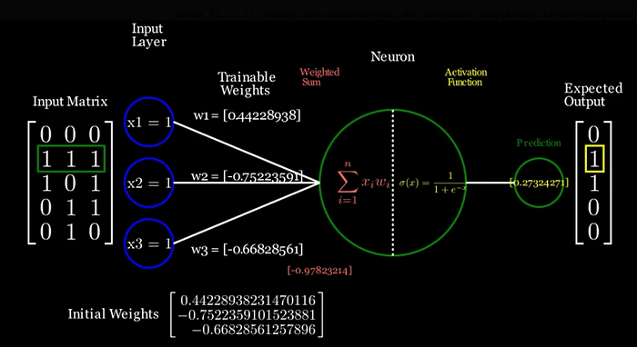
After enough training iterations, the perceptron will adjust its weights to minimize the error for all training samples. In a simple problem that is linearly separable, one neuron can eventually learn to map inputs to the desired outputs by finding an appropriate linear decision boundary.

Note: A single perceptron can only learn a linear relationship between inputs and output. If the task is not linearly separable (like the XOR function), a single neuron won’t suffice. This limitation is why we introduce hidden layers (making a multilayer perceptron) with non-linear activation functions to tackle complex patterns. But even in multi-layer networks, the fundamental unit remains neurons with weights learned via the same principle.

Scaling Up: From One Neuron to Millions (and Billions)

The perceptron example has only a handful of parameters (3 weights, and maybe 1 bias) — essentially on the order of 10⁰ to 10¹ parameters. Modern neural networks, however, consist of many neurons layered together, so their parameter counts explode. For instance, a modest multilayer perceptron (MLP) with one hidden layer of 10 neurons taking 3 inputs would have 3 X 10 + 10 X 1 = 40 weights (plus biases), which is already an order of magnitude more. As we stack more layers or increase width, the count grows multiplicatively.

Transformers, introduced in 2017, are a deep learning architecture that takes scaling to a different level. They are the backbone of today’s large language models. A transformer isn’t just one neuron — it’s a whole network chunk composed of many neurons and linear operations, repeated in layers. Let’s break down a single transformer block in comparison to our single perceptron:

• Inputs: In a perceptron we feed in raw features (e.g., numeric values). In transformers for text, the inputs are first converted to embedding vectors (these embeddings are themselves produced by weights — an embedding matrix plays a role analogous to input weights, mapping a token ID to a vector representation).

• Linear transformations: A perceptron computes one weighted sum. A transformer block computes multiple linear combinations of its inputs. In the self-attention mechanism, for example, each token’s embedding is linearly projected into three different vectors: Query (Q), Key (K), and Value (V). These are obtained by multiplying the embedding by three weight matrices W^Q, W^K, W^V. Those matrices are learned parameters just like perceptron weights. Instead of a single weighted sum, the transformer uses these to calculate attention scores and weighted sums of values — effectively a learned way to weight inputs dynamically rather than fixed weights to a single output.

• Activation function: Our perceptron used a sigmoid. Transformers use more complex functions. After the self-attention step, a transformer block has a feed-forward network (FFN) component: this is basically two layers of neurons applied to each position’s data. The FFN introduces nonlinearity (often using ReLU or GELU activation) and further mixes information. The weights in the FFN are also parameters that get trained (and notably, a large fraction of a transformer’s parameters lie in these feed-forward layers).

• Outputs: A perceptron outputs a single value. A transformer block outputs an enhanced set of embeddings (same number of tokens as input, but each altered by attention and the FFN). Stacking many such blocks (each with their own sets of weight matrices) produces the final representation, which then might go through an output layer to generate a prediction (e.g., the next word probabilities in a language model).

In essence, if you zoom out, a transformer is doing what a perceptron does — but at a vastly larger scale and with clever architecture. Both systems multiply inputs by weights, apply activations, and adjust weights through training. The transformer just has many more weights and a structured way of connecting them.

Parameter Growth from Perceptrons to GPT-3

To grasp the scale difference, let’s compare the number of parameters (trainable weights) in various models:

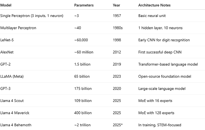
As the table shows, model sizes have increased exponentially. GPT-3’s 175 billion parameters dwarfs earlier networks by many orders of magnitude. Each of those parameters is a weight (or bias) in some layer of the neural network. They are organized into matrices and tensors within the transformer architecture (for example, GPT-3 has dozens of layers, each with many attention heads and feed-forward neurons, all contributing to that total).

Yet, how are those 175 billion parameters learned? Surprisingly, in essentially the same way as our perceptron’s 3 weights were learned. Of course, we don’t train GPT-3 by hand-coding a loop in pure Python — instead, we use highly optimized distributed training with backpropagation. But conceptually, the training loop still iteratively adjusts the model’s weights to reduce error (or more precisely, to minimize a loss function) using algorithms like gradient descent. The difference is scale and complexity of data:

• A perceptron might be trained on a few dozen examples (small data, manual loop).

• GPT-3 was trained on 45+ terabytes of text data, using massive compute clusters — but the training still involved feeding examples (chunks of text), computing outputs and errors, and nudging weights repeatedly (billions of times) to fine-tune the predictions.

Conclusion

From a single perceptron to a 175-billion-parameter transformer, the journey of neural networks is one of scaling up parameters and architecture while staying true to the same fundamental learning mechanism. By understanding one perceptron’s learning process — inputs weighted and summed, passed through an activation, and adjusted via error feedback — you’ve essentially understood the nugget of how even the most sophisticated large language models learn. Modern transformers are just a vast collection of perceptron-like units working in concert. Each weight in GPT-3 plays a small role, but collectively they enable incredible capabilities. And as you continue your ML journey, remember: today’s magical LLMs are, at their heart, doing lots and lots of what a single neuron does, just on a grander scale.

References:

1. Wikipedia — GPT-3, model description and parameter count.

2. Quanta Magazine (via Wired) — Discussion of LLM scaling and parameters (GPT-2 at 1.5B, GPT-3.5 at 350B)wired.com.

3. Labellerr Blog — LLaMA models (7B to 65B parameters) and their design considerationslabellerr.com.

4. Anushka Sonawane, “Query, Key, Value and Multi-Head Attention: Transformers Part 2,” Medium — explanation of Q, K, V weight matrices as trainable linear layers.

5. Marquee Insights — “AI Explained — Model Training…” — on model training and parameters (weights & biases, example of GPT-3’s 175B).