Image Processing: Photo Editor From Scratch (Part 1)

In this project, I created a fully functional image editor using Python, NumPy, and Tkinter — with no dependency on heavy libraries like OpenCV or PIL for the core image processing.

The editor includes features like:

• Brightness, Contrast, and Saturation controls

• Auto-enhancement

• Sharpening, Blur effects, and Seasonal filters

• Artistic effects like Crayon and Pencil Sketch

In this blog post, I’ll first explain the image processing concepts and underlying math — including how pixel manipulation works using NumPy arrays. Then, I’ll walk you through the actual code implementation, covering how these features come together in a desktop GUI built with Tkinter.

I. Intro

Image processing is a foundational of modern Artificial Intelligence and Machine Learning in Computer Vision.

Before machines can “understand” images, they need to see them in a structured way — and that’s where image processing comes in.

Here’s why it matters:

• Preprocessing for ML Models: Clean, enhanced, and normalized images are crucial for training accurate models. Techniques like contrast adjustment, sharpening, and de-noising can significantly improve performance.

• Feature Extraction: Image filters (e.g., edge detection, blurring, thresholding) help extract meaningful patterns that models can learn from, such as object shapes, textures, or boundaries.

• Data Augmentation: Image transformations like brightness variation, blur, and artistic effects are used to generate diverse training datasets and make models more robust.

• Real-World Applications: From facial recognition and medical imaging to autonomous vehicles and OCR, nearly every AI-driven visual system relies on efficient image processing as a critical first step.

II. Fundamentals

In the digital world, an image is simply a matrix of numbers — a structured grid where each number represents the intensity of light at a specific point, called a pixel.

1. Grayscale (Black & White) Images

A grayscale image can be represented as a 2D matrix:

• Each element (pixel) holds a value between 0 and 255, where:

  • 0 = pure black

  • 255 = pure white

  • Values in between represent varying shades of gray.

For example, a 100×100 grayscale image is stored as a 100×100 NumPy array.

2. Color Images (RGB)

Color images are slightly more complex. They use three channels:

• Red, Green, and Blue (RGB)

• Each channel is a separate 2D matrix of intensity values from 0 to 255.

So, a color image is a 3D NumPy array of shape: (height, width, 3). Each pixel in a color image is a triplet of values: [R, G, B] — for example, [255, 0, 0] means pure red.

3. Point Processing

Point processing is the application of mathematical functions to pixel values. You can think of a pixel transformation as a function:

$$T(r) = s$$

Where:

• r is the scalar input intensity of a pixel (or group of pixels)

• T is the image processing operation (like blur, sharpen, brighten, etc.)

• s is the output of transformed pixel intensity value

In simple terms:

We take each pixel intensity value, apply a transformation function T(r), and replace it with the result.

Examples:

Brightness Adjustment:

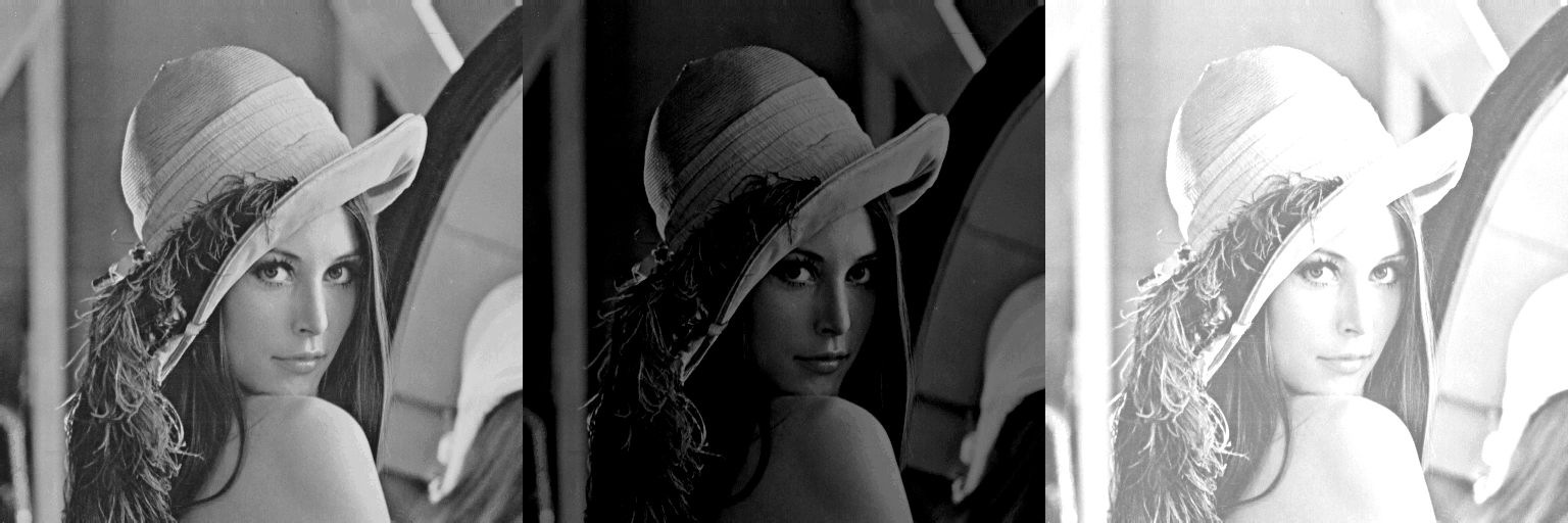
Add a constant to every pixel to make the image brighter or darker.

Contrast Stretching:

Let input intensity be r, and output be s = f(r). The transformation is defined as:

$$f(r) = \begin{cases} \frac{s_1}{r_1} \cdot r, & 0 \leq r < r_1 \\ \frac{s_2 - s_1}{r_2 - r_1} \cdot (r - r_1) + s_1, & r_1 \leq r \leq r_2 \\ \frac{255 - s_2}{255 - r_2} \cdot (r - r_2) + s_2, & r_2 < r \leq 255 \end{cases}$$

Enhance contrast by stretching the intensity range [r1, r2] to [s1, s2].

This creates a 3-part linear function:

• Low intensities (0 to r1) are stretched to 0 to s1

• Mid-range intensities (r1 to r2) are stretched to s1 to s2

• High intensities (r2 to 255) are stretched to s2 to 255

4. Spacial Domain Filtering ( Convolution )

Spatial filtering is a technique in image processing where each pixel’s value is modified based on its neighborhood using a filter/kernel (a small matrix).

This calculation is done using convolution, which involves:

• Sliding the kernel over the image, pixel by pixel.

• At each position, computing a sum of products between the kernel values and the corresponding image pixel values.

• The calculation is performed row by row, and within each row, column by column.

• For each row offset i, you compute across all column offsets j, applying the kernel over the local image region. For example, with a 3×3 kernel, you compute the sum of element-wise products between the 3×3 kernel and the 3×3 image region it overlaps. The result replaces the center pixel of that region.

$$g(x, y) = \sum_{i=-a}^{a} \sum_{j=-b}^{b} w(i, j) \cdot f(x+i, y+j)$$

Where:

• f(x, y): input image (intensity at pixel (x, y))

• g(x, y): output image at pixel (x, y)

• w(i, j): kernel/filter weights at offset (i, j) from the current pixel (x, y)

• m × n: kernel size (usually odd like 3×3, 5×5)

• a = ⌊m/2⌋ → Half of the kernel height, b = ⌊n/2⌋ → Half of the kernel width

Example:

Median Filter:

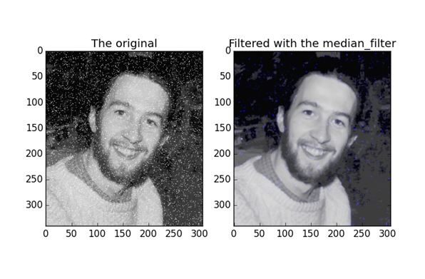
$$ w = \frac{1}{9} \begin{bmatrix} 1 & 1 & 1 \ 1 & 1 & 1 \ 1 & 1 & 1 \ \end{bmatrix}$$

Smooths the image by replacing each pixel with the average of its neighbors.

5. Frequency Domain Filtering ( Fourier Filtering )

Filtering in the frequency domain involves modifying an image by transforming it into frequencies, altering those frequencies, and transforming it back.

a) Fourier Transform

The Fourier Transform converts an image from the spatial domain (pixels) into the frequency domain, representing the image as a sum of sinusoidal patterns with different frequencies and amplitudes.

• It breaks down the image into its frequency components.

• Each frequency component shows how quickly pixel values change in a particular direction.

• Low frequencies correspond to smooth, slowly changing areas; high frequencies correspond to edges and fine details.

b) Filtering

Frequency domain filtering modifies an image by applying a mask (filter) to its frequency representation.

Steps:

1. Fourier Transform the image to get the frequency spectrum.

2. Apply a mask (e.g., low-pass, high-pass) — a matrix that keeps or blocks certain frequencies.

   • Multiply the frequency image with the mask.

3. Inverse Fourier Transform the result back to the spatial domain.

Example:

Gaussian Filter:

$$ H(u, v) = e^{- \frac{D(u, v)^2}{2D_0^2}}$$

• H(u, v): filter value at frequency point (u, v)

• D(u, v): distance from center of the frequency image

$$D(u, v) = \sqrt{(u - M/2)^2 + (v - N/2)^2}$$

• D_0: cutoff frequency (controls blurriness)

• M, N: size of the image

Explain:

• Center of the frequency image = low frequencies → retained (value ~1)

• Outer parts = high frequencies → suppressed (value ~0)

This gives a smooth blur without sharp cutoffs like ideal filters.

Steps:

1. Take Fourier Transform of the image → F(u, v)

2. Create Gaussian low-pass mask H(u, v)

3. Multiply:

$$G(u, v) = F(u, v) \cdot H(u, v)$$

4. Take Inverse Fourier Transform → g(x, y)

III. Up Next:

In the next part, we’ll show a code implementation and explanation of some of the features of the photo editor in Python and NumPy.