Choosing the optimal database for your application involves understanding the strengths of different database categories. Below we break down several major types of databases, explaining each in simple terms, when to use them, key design considerations, and examples of popular systems in each category. This structured guide will help you match your use case to the right kind of database technology.

1. Relational Databases (RDBMS)

1.1 What It Is

Relational databases store data in structured tables with rows and columns, much like a spreadsheet. Each table has a defined schema (a fixed set of columns), and tables can be linked via relationships. For example, a business might have a Customers table and an Orders table, where each order references a customer by an ID. This model lets you use SQL (Structured Query Language) to query and join data across tables. Relational systems enforce data integrity through rules like primary keys (unique identifiers for rows) and foreign keys (links between tables). They also support ACID transactions — ensuring operations are Atomic, Consistent, Isolated, and Durable — which guarantees reliability for multi-step updates (e.g. transferring money between bank accounts).

1.2 When to Use It

Use a relational database when your data is highly structured and integrity is critical. They shine for transactional systems where you need strong consistency and the ability to combine data from multiple tables in one query (complex joins). Examples include financial systems, inventory and order management, or any scenario where it’s essential that all parts of a transaction succeed together. Relational databases are optimized for operations that affect multiple records across different tables with consistency (for instance, processing an order might update inventory, orders, and payments tables in one go). If you need multi-row transactions or complex queries across structured data (such as reporting sales by region and product), a relational RDBMS is often the right choice.

1.3 Key Design Considerations

Schema Design: You must define a schema upfront. Organize data into tables and relationships (normalization) to reduce duplication. Changing the schema (adding columns or tables) later can be involved, so anticipate future needs.
ACID Transactions: Relational DBs ensure strong consistency via ACID, which is great for reliability. However, ensuring ACID compliance can introduce overhead that may impact performance in very high-throughput scenarios.
Scaling: Traditional RDBMS scale vertically (adding hardware resources to one server) or through read-replicas. Sharding (horizontal partitioning) is possible but adds complexity. They are not built for massive horizontal scale-out as easily as some NoSQL systems, so very large applications might need to invest in careful sharding or use cloud variants (like distributed SQL databases). You can refer to the following in-depth article on how to scale MySQL horizontally: Scaling the Data Layer with MySQL — A Detailed Exploration. It covers architectural patterns, sharding strategies, replication, and best practices for building a resilient and scalable MySQL-based backend.
Performance Tuning: Proper indexing is crucial for performance. You need to design indexes on columns used in filters/joins. Also consider caching frequent queries and using database tuning techniques for speed.
Rigidity vs. Flexibility: The fixed schema and strong consistency bring predictability, but at the cost of flexibility. If your data model changes frequently or the data is unstructured, a relational DB might slow down development due to migrations and strict schemas.

1.4 Popular Databases

MySQL — A widely used open-source relational database, great for web applications.
PostgreSQL — An open-source RDBMS known for advanced SQL features and extensions (e.g. PostGIS for spatial data).
Oracle Database — A commercial enterprise RDBMS with extensive features for large systems.
Microsoft SQL Server — A robust enterprise RDBMS commonly used in Windows/.NET environments.

2. In-Memory Databases

2.1 What It Is

In-memory databases are designed to keep data primarily in RAM (memory) rather than on disk. By avoiding slow disk I/O, they provide extremely fast data access. They often serve as caches or real-time data stores. In-memory systems can respond in microseconds or milliseconds, even under high load.

Applications that demand real-time responsiveness, such as gaming leaderboards or live analytics dashboards, often leverage in-memory databases to ensure that data — like scores or metrics — updates instantly for end users. These systems benefit from ultra-fast access times by keeping data in RAM instead of disk. In fact, high QPS (Queries Per Second) systems — including ad platforms, payment gateways, and recommendation engines — commonly adopt in-memory databases to handle massive volumes of read and write operations with minimal latency. These databases might still persist data to disk in the background or via snapshots, but reads and writes hit the in-memory dataset for speed.

2.2 When to Use It

Use an in-memory database when speed is critical, and either you can tolerate data loss on restart or have a mechanism to reload or persist the data.

In many real-world architectures, the system starts in a “cold” state, where data is loaded from a persistent store (like a relational DB or file system) into the in-memory cache during initialization. Once the required data is cached (sometimes referred to as “warming up the cache”), the system begins serving requests directly from memory, ensuring low latency and high throughput.

This hybrid approach combines the durability of traditional databases with the performance of in-memory systems. Frameworks like Apache Ignite, Redis (with persistence or cache-loader modules), and Hazelcast support such configurations out of the box.

Common use cases for in-memory databases include:

Caching: Storing frequently accessed data — such as session tokens, user profiles, or pre-rendered page fragments — to reduce response times and database load. Web applications often cache results of expensive queries or frequently accessed content to efficiently handle high traffic.
Real-Time Analytics: Applications that perform rapid calculations on streaming data (e.g., fraud detection, risk analysis, live dashboards, or IoT telemetry) use in-memory databases to ingest, analyze, and react to data on the fly with minimal latency.
Gaming and Leaderboards: Online multiplayer games use in-memory storage to maintain real-time leaderboards and game states. This ensures instant updates for player scores, positions, or achievements across all clients.
Payment Systems: High-throughput payment gateways and transaction processing platforms use in-memory databases to temporarily store transaction states, rate-limiting information, or fraud detection flags — helping them maintain ultra-low latency under peak loads while syncing to a durable store in the background.
Message Queues and Event Buffers: In-memory stores like Redis Streams or Apache Ignite queues are often used to buffer high-velocity data streams or events, acting as lightweight intermediaries before data is processed or persisted elsewhere.
Handling Traffic Spikes: Systems that experience sudden surges in usage — such as flash sales, breaking news, or viral content — leverage in-memory data layers to absorb the load gracefully. Memory-based systems can process thousands of operations per second, helping to maintain user experience during spikes.

2.3 Key Design Considerations

Volatility and Durability: Data in RAM is volatile — if the server loses power, data can be lost. Many in-memory databases offer persistence options (like snapshotting to disk or append-only logs), but writing to disk can slow things down. Decide if the data is ephemeral (e.g. cache or session that can be recomputed) or if you need backups/replication for safety. Often, caching layers sacrifice some durability for speed.
Memory Capacity: RAM is more expensive and limited than disk storage. Ensure the dataset can fit in memory, or plan for strategies like data eviction (e.g. least-recently-used eviction in a cache) when memory fills up. If your data grows very large, an in-memory solution might become cost-prohibitive.
Scaling and Clustering: In-memory databases can be distributed across multiple nodes (sharded) to increase capacity and throughput. Consider how the system handles clustering — for example, sharding by key or using consistent hashing. Network overhead can become the bottleneck when scaling out, so monitor latency.
Data Structures and Features: Some in-memory stores (like Redis) offer special data structures (lists, sets, sorted sets, etc.) that let you perform complex operations in memory efficiently. Designing your use of these data structures can greatly affect performance and memory usage.
Use with a Persistent DB: Often, in-memory DBs are used alongside a persistent database. For instance, an application might first check the in-memory cache for a value and fall back to the relational database if not present. Make sure to have cache invalidation strategies in place so that the in-memory layer doesn’t serve stale data when the source of truth updates.

2.4 Popular Databases

Redis — A popular in-memory key-value store known for its speed and support for various data structures. Often used for caching, real-time analytics, and pub/sub messaging.
Memcached — A lightweight in-memory cache primarily for simple key-value string data; commonly used to speed up web applications by caching query results.
Apache Ignite — An in-memory data grid that can distribute data across a cluster, offering SQL querying and processing in memory.
SAP HANA — An in-memory relational database for enterprise use, enabling fast analytics on large datasets (often used in enterprise analytics and data warehousing).

3. Key-Value Databases

3.1 What It Is

Key-value stores are a simple yet powerful type of NoSQL database that store data as a collection of key–value pairs, much like a dictionary in Python or a hash map in Java.

Each key acts as a unique identifier, and the associated value can be a simple data type (like a string or number) or a more complex object (like a JSON document), or even a blob of data. This structure allows for fast lookups, making key-value stores ideal for use cases like caching, session management, user preferences, and real-time counters.

This simplicity lets key-value stores achieve high performance and flexibility. For example, you might use a key-value database to store user preference settings, where the key is the user’s ID and the value is a blob of settings data for that user. The database simply stores and returns the value given the key, without needing to know the internals of that value.

Note: While key-value databases and in-memory databases may appear similar — especially since many in-memory systems use a key-value structure — there is a fundamental difference in how they are classified*. A **key-value database is categorized based on its data model — it focuses on the format and structure of how data is organized, specifically as key–value pairs. In contrast, an in-memory database is classified based on its storage medium — it focuses on where the data is stored*, namely in *RAM*, to deliver extremely fast access. So, while an in-memory database might use a key-value format internally, the two are fundamentally different in philosophy: *key-value relates to data format*, whereas *in-memory relates to data storage strategy.*

3.2 When to Use It

Use a key-value database when you need fast, simple lookups by key and you don’t require complex querying on the data. They are ideal for scenarios like:

Caching and Session Storage: Key-value stores excel at caching results or storing user session data (keyed by session ID or user ID) for quick retrieval. This speeds up web applications by avoiding repeated computations or database joins.
High-Throughput Scenarios: When you need to handle a massive number of small reads/writes (e.g. handling millions of simple queries per second), key-value stores are very effective. They are easy to distribute across multiple servers by partitioning keys, so they can scale horizontally to handle huge workloads. Large web services and gaming backends often use key-value stores to manage state.
Simple Configurations or Feature Flags: Storing configuration data or feature flag values that your application looks up by key. For instance, an application might store feature toggles in a key-value DB where each feature name is a key and the value indicates if it’s on/off for a given user segment.
Event or Log Processing Pipelines: Sometimes key-value stores are used as buffers or last-seen trackers in event processing. For example, keeping track of the last processed event ID per user in a key-value store for a streaming system.
When Flexibility is Needed: If your data does not fit a fixed schema or may vary from item to item, key-value can store it without requiring upfront definition. (If you need to query inside the data, though, a pure key-value store won’t help — consider a document DB in that case.)

3.3 Key Design Considerations

Data Model Simplicity: Key-value databases don’t support complex queries or relationships. You design your application to know the key for any piece of data you want. If you need to retrieve data by something other than the primary key, you may need to maintain secondary indexes in another system or as additional key-value entries (e.g. store reverse lookups).
Partitioning (Sharding): These stores naturally partition by key, which makes horizontal scaling straightforward. However, you should choose keys carefully to avoid “hot spots.” For example, using timestamps or sequential IDs as keys can direct too much load to one shard; better hashing or randomization of keys can distribute load evenly.
Consistency: Some key-value systems (especially distributed ones) opt for eventual consistency to maximize availability. This means a recent update might not be visible to all replicas immediately. If you use a clustered key-value store (like DynamoDB or Riak), consider the consistency settings — you might get faster writes at the cost of reads possibly seeing slightly stale data.
Data Size Limits: Often, there are practical size limits per value (e.g. many key-value stores handle values up to a few MB efficiently). Storing very large blobs might not be ideal in a key-value store (a dedicated blob store could be better for huge files).
Memory vs Disk Storage: Some key-value databases are in-memory (like Redis, Memcached) which gives speed but requires memory and may lose data on restart. Others (like RocksDB-based or DynamoDB) store on SSD/disk for durability. Decide based on whether persistence is required or it’s purely a cache.
Lack of Transactions: Typically, key-value stores operate on single records. If you need multi-key transactional updates (updating two keys together reliably), support for that is limited. Some systems provide limited transactions or batch operations, but it’s not as seamless as in relational databases.

3.4 Popular Databases

Redis — (Fits here as well) A versatile in-memory key-value store, often used for caching, pub/sub messaging, counters, and more.
Memcached — (Also fits here) A simple, high-performance in-memory key-value cache, commonly used to speed up web apps.
Amazon DynamoDB — A fully managed cloud key-value database that scales horizontally; offers high throughput and optional consistency controls (inspired by Amazon’s Dynamo paper).
Riak KV — An open-source distributed key-value store known for its fault tolerance and eventual consistency model.
(Many systems like Redis and Memcached are both key-value and in-memory; we list them in both categories as they are quintessential examples.)

4. Full-Text Search Databases

4.1 What It Is

Full-text search databases (or search engines) are specialized systems optimized for searching and indexing text content. Instead of treating data as structured rows or simple key-value pairs, they create inverted indexes on the text, which allow quick look-ups of documents containing specific words or phrases. In a full-text search database, you can ask complex questions like “find documents that contain words similar to database and index near each other.” The engine will return results sorted by relevance, using algorithms to determine how well each document matches the query. This is much more advanced than a SQL %LIKE% query. A full-text search database examines all the text in documents to find matches to a user’s search terms. For example, if you run an e-commerce website, you might use a full-text search engine to power the product search box. When a user searches for "wireless headphones noise cancelling", the search engine can quickly return products whose descriptions or reviews match those terms, even ranking them by relevance.

4.2 When to Use It

Add a full-text search database when your application needs robust search capabilities on large amounts of text. Common scenarios include:

Website or Document Search: If your app stores articles, documents, product descriptions, or any long text, a search DB allows users to find information by keyword, phrase, or even fuzzy matches. For example, a documentation site or a knowledge base would use this so users can search by topic.
Logs and Event Data: Log management systems often use full-text indexing (with time filters) so that engineers can search error logs for specific messages or keywords quickly.
E-commerce Product Search: As mentioned, to let customers search by product name, category, or features. A full-text engine can handle varied queries (with typos, plural/singular forms, etc.) and still find relevant items.
Enterprise Search: Searching across many internal documents, emails, or records. Full-text search can index across different sources to provide unified search results.
Anywhere Keyword Search is a Feature: Forums, social media, job listings, and other platforms with user-generated text often incorporate a search engine so users can find posts or entries containing certain terms.

Many organizations introduce a search engine alongside their primary database specifically to handle these text queries efficiently. If users expect a search box or filtering by text in your app, a full-text search backend is likely needed.

4.3 Key Design Considerations

Indexing Overhead: Building and maintaining indexes on large text fields can consume significant CPU, memory, and storage. There’s a trade-off between index size and query speed. You may need to fine-tune what you index (e.g. maybe you index product names and descriptions, but not every log field). Also, updating indexes (when data changes) incurs overhead; some systems do near-real-time indexing, others batch updates for efficiency.
Relevance Tuning: Full-text systems score results by relevance. You might need to tweak ranking algorithms or boost certain fields (for instance, matches in a title might be more important than matches in a body text). This can be a complex aspect — expect to adjust settings or use analytical tools to improve search result quality for your users.
Distributed Search: Search databases often run as clusters (sharding index by document or by term). Ensure you have a strategy for scaling as data grows — e.g., adding shards and replicas. Also, note that executing a single search query may hit multiple shards and then aggregate results, so network and coordination costs matter.
Handling of Data Changes: If your primary data (in a relational or document DB) updates, how will those changes reflect in the search index? Often there’s an eventual consistency model — the search index might not update the instant data changes. You may need to design a pipeline to feed changes (like using Kafka or change data capture) into the search system.
Text Analysis Features: Decide how to utilize features like stemming (so searching “runs” finds “running”), stop words (ignoring common words like “the”), synonyms, and support for multiple languages. Full-text engines typically let you configure analyzers for different languages and use cases. Choose the right analysis pipeline for your text to balance recall (finding all relevant results) vs precision (only highly relevant results).
Security and Privacy: If you index sensitive data, remember that search indexes are another copy of your data. Secure them properly. Also, implement search authorization if needed (so users only see results they have permission to view).

4.4 Popular Databases

Elasticsearch — A distributed full-text search engine based on Lucene, commonly used for logging, search on websites, and analytics. It offers powerful querying and aggregation capabilities.
Apache Solr — An open-source search platform also built on Lucene, often used for enterprise search and e-commerce search platforms (Solr powers search for some large websites).
OpenSearch — A community-driven fork of Elasticsearch (maintained by Amazon) that provides similar full-text search features in an open-source manner.
Algolia (service) — A hosted search-as-a-service solution that provides full-text search with an emphasis on speed and typo-tolerance (often used in websites and mobile apps for instant search results).
(Lucene is the underlying library behind many of these, but Elasticsearch and Solr are the user-friendly servers built on it.)

5. Document Databases

5.1 What It Is

Document databases store data in documents, typically formatted as JSON or XML, rather than in fixed tables. A “document” is a self-contained data entry that can have a flexible structure — different documents in the same collection can have different fields. These systems are schema-less; you don’t define all the fields upfront. For example, imagine a user profile document: one user’s document might have fields for name, email, and 3 phone numbers, while another user’s document has name, email, and an array of social media accounts. Document databases can store both of these in the same collection without issues. Internally, they treat the document as a tree of nested key-value pairs (like a JSON object with sub-objects). Unlike a pure key-value store, the database understands the structure of the document, so you can query based on nested fields (e.g. find all users where address.city = "London"). This ability to exploit the document’s internal structure allows more powerful queries than a flat key-value store.

Note*: A **key-value store is the simplest type of NoSQL database. It stores data as individual key–value pairs*, where the key is a unique identifier and the value is usually a blob (binary or JSON, for example) that the database does not interpret. You can only retrieve or update the entire value by key — *there’s no understanding of the structure inside the value**. It’s like a black box: fast and simple, but limited in querying capabilities.*

A document data store*, on the other hand, also uses keys to identify data, but the values are **structured documents*, typically in *JSON, BSON, or XML*. Unlike key-value stores, document databases *understand the internal structure of the document**, allowing you to query, filter, or update specific fields within a document using rich query languages. You can index individual fields, perform nested searches, and even run aggregations.*

5.2 When to Use It

Consider a document database when your data is semi-structured or you need flexibility in your schema. Use cases include:

Content Management and Blogging: Each article or post can be a JSON document with its title, body, tags, comments, etc. Different posts might have additional fields (one might have an array of images, another might have a video link), and a document DB will happily store them without schema changes. Many CMS and blogging platforms use document stores for this reason.
User Profiles and Catalogs: Applications where each record might have a varying set of attributes. For instance, an e-commerce product catalog — one product might have size and color fields, another might have dimensions and weight. Storing each product as a document allows flexibility as the product specs vary. Similarly, user profile data that can easily extend with new preferences or settings is a good fit.
Event Logs and Sensor Data: Each event can be a JSON document (with a timestamp and various attributes). Different events might have different schemas. Document DBs can store these without a predefined schema, and you can query by attributes present in those events.
Rapid Development with Evolving Schema: If you’re iterating quickly and adding new features that require storing new fields, a document DB lets you add those fields on the fly in the code without migrations. Startups and agile teams might prefer this flexibility early on.
Geographically Distributed Data: Some document databases (like CouchDB/Couchbase) are designed to sync data across devices or regions, which is useful for apps that need offline-first capabilities (e.g. a mobile app that stores user data locally as documents and syncs when online).

Additionally, document databases scale out well for read/write throughput by distributing documents across shards in a cluster. This makes them suitable for large-scale applications where a relational database might become a bottleneck or too rigid.

5.3 Key Design Considerations

Data Modeling — Embed vs Reference: In document design, you often have a choice: embed related data in one document or keep them in separate documents. For example, store an order and its line items together in one order document (embed), or have an orders collection and a separate order_items collection (reference). Embedding can make reads faster (one document fetch) at the cost of potential duplication, whereas referencing keeps data normalized but requires multiple queries. Design your documents based on how your application queries the data (generally favor embedding for one-to-few relationships that are retrieved together, and referencing for truly large or independent sub-objects).
Indexing: Just like relational databases, document DBs allow indexes on fields to speed up queries. Be mindful to create indexes on fields you will filter or sort on frequently (e.g., an index on email or last_login if you query by those). Too many indexes can slow down writes, though, and unlike a fixed schema, if many documents have a field but some don’t, indexing that field still indexes the subset of documents that have it.
Joins and Multi-Document Operations: Document databases typically don’t support joins across collections like SQL does (some have limited join-like aggregation, but it’s not their strong suit). If your use case requires combining data from multiple document types frequently, you might end up doing those joins in application code or using multi-step queries. Also, transactions in many document DBs are scoped to a single document. Newer versions of some (e.g. MongoDB) do support multi-document transactions, but using them heavily can reduce the advantage of the database’s performance.
Schema Evolution: Although schema-less, you still need to manage changes. Your code must handle cases where a field might be missing or an old field is present in some documents. It’s a good practice to have versioning or migration strategies for your documents if your data model changes significantly (e.g. you might update all docs to a new structure in the background, or handle both old/new formats in code).
Consistency and Sharding: In distributed document DBs, you often choose a shard key (maybe a user ID or some category) that decides how documents are distributed. Picking a good shard key is important to avoid uneven load. Also, consider the consistency model — many document databases default to eventual consistency in a cluster for better performance, but often allow configuring writes to be replicated to multiple nodes (at the cost of write latency) if stronger consistency is needed.
Query Capabilities: Document stores allow rich queries (on nested fields, array contents, etc.), but complex aggregations or analytics across huge data sets may not be as fast as in specialized analytical databases. Some document DBs provide aggregation frameworks (like MongoDB’s aggregation pipeline) which are powerful, but you need to be mindful of performance on very large data or consider using additional analytics tools for those cases.

5.4 Popular Databases

MongoDB — The most popular document database, storing JSON-like BSON documents. It’s known for its developer-friendly query language and scalability. Frequently used in web applications and known for the MEAN/MERN stack (where MongoDB is the “M”).
Couchbase — A distributed document database that also offers in-memory caching and full-text search integration. It’s designed for high performance at scale and can sync with mobile (Couchbase Mobile).
Apache CouchDB — An open-source document store famous for its replication and sync capabilities (e.g. allowing offline-first applications with eventual sync). It stores JSON documents and has a RESTful HTTP API.
Azure Cosmos DB (SQL API) — A globally distributed multi-model database; its SQL API is essentially a document store for JSON data (compatible with MongoDB in many ways). It offers tunable consistency and is used for high availability across regions.

6. Graph Databases

61. What It Is

Graph databases are built for data that is all about relationships. Instead of tables or isolated documents, a graph database represents information as a network of nodes and edges. Nodes are entities (e.g. a person, a product, a city) and edges are the connections or relationships between those entities (e.g. “Alice FOLLOWS Bob” in a social graph, or “City A –> City B flight route”). Both nodes and edges can hold properties (attributes) describing them. This structure is very flexible and naturally models complex interconnected data. A graph database excels at traversing these connections quickly — for example, finding all of someone’s friends-of-friends in a social network, or the shortest path in a map of cities. Because relationships are stored as first-class citizens, queries that would be Joins in SQL (and get very expensive as they chain together) can be performed more directly in graph DBs. In short, graph databases make it easy to answer questions about how things are connected. For instance, you could query a graph DB: “Give me recommendations of products that are liked by people who are similar to me” — the database can traverse the “likes” relationships and “similar to” relationships efficiently to produce results.

6.2 When to Use It

Use a graph database when your data is richly connected and you need to frequently explore or analyze those connections. Scenarios include:

Social Networks: This is a classic use. Users (nodes) connect to other users with relationships like friendships or follows. Graph DBs can easily find mutual friends, degrees of separation, or influencers (nodes with many connections) in the network.
Recommendation Engines: Many recommendation systems can be viewed as a graph problem — connecting users to products to categories, or users to other similar users. A graph DB can find, for example, products that a user might like based on the interests of users they are connected to or have similarity with.
Fraud Detection: In financial or insurance industries, graph analysis helps detect fraud rings. Each person, account, or transaction can be a node, and edges can represent transfers or shared info. By traversing, you might discover that multiple seemingly unrelated claims or accounts connect to the same phone number or IP address, revealing a fraud network.
Knowledge Graphs & Semantic Queries: For modeling knowledge domains (like an encyclopedia of entities and how they relate: a graph of actors, movies, directors, etc.), graph DBs let you store complex relationships and query them (e.g. “Find all actors who have worked with a particular director through at most two movies”). This is used in things like Google’s Knowledge Graph to enhance search results with related info.
Network/IT Operations: Representing computer networks, transportation routes, or supply chains. Graphs can answer connectivity and path questions: “If this router fails, what systems are impacted?” or “What’s the optimal route or dependency chain between these two points?”
AI and Recommendations (RAG): Recently, graphs are even used to augment AI applications — for example, connecting concepts in a graph can help a Retrieval-Augmented Generation system find context for an AI to use. In general, if your application benefits from discovering indirect relationships or patterns in connections, graph DBs are useful.

6.3 Key Design Considerations

Data Volume and Distribution: Graph databases perform best when a substantial portion of the graph can be kept in memory and traversals can hop quickly from node to node. If you have a massive graph (billions of nodes/edges), you may need to distribute it, but distributing a graph is tricky — traversals that cross partition boundaries can become slower. Some graph databases are optimized for sharding, but many production graph use-cases are solved on a single powerful machine or a small cluster to keep traversals fast. Consider how your graph might partition (e.g. by sub-graph communities) if it grows huge.
Query Patterns: Think about the questions you’ll ask. Graph query languages (like Cypher for Neo4j, or Gremlin, etc.) allow pattern matching (“find nodes of type X connected via Y to nodes of type Z”). Ensure your data model (node and edge labels, properties) is designed to answer those efficiently. Use indexes on node properties that you frequently use as starting points in traversals (many graph DBs let you index certain attributes to find starting nodes quickly, before traversing relationships).
Updates and Consistency: If relationships change frequently (e.g. constantly adding/removing edges), consider the performance of writes. Some graph DBs can handle heavy transactional updates, but it’s a different pattern than append-only logs or document inserts. Also, if using a cluster, consider how it ensures consistency of relationships across nodes — often a single-edge update might be transactional, but updating many edges (like removing a node and all its connections) should be done carefully.
Algorithmic Complexity: Graph traversals can inadvertently touch a lot of nodes if queries aren’t tight. For instance, a naive query for friends-of-friends-of-friends in a dense network can explode in complexity. You may need to put limits or depth bounds on queries or use algorithms (many graph DBs come with built-in graph algorithms for centrality, shortest path, etc.). Leverage those instead of writing huge traversals yourself when possible.
Integration with Other Data: Often, graph databases are used alongside other databases. You might keep core relational data in an RDBMS but use a graph DB for specific recommendation queries. Keeping the data in sync (or deciding which is the source of truth) is important. Some multi-model databases (like Cosmos DB with Gremlin API, or ArangoDB) try to offer both document and graph models to reduce duplication. Evaluate if a multi-model approach suits you or if you’ll maintain separate systems.
Learning Curve: Querying a graph is different from SQL. If your team is new to graph databases, there’s a learning curve for the query language and the way of thinking (it’s more about pattern matching than set-based logic). Plan for some ramp-up time.

6.4 Popular Databases

Neo4j — The most well-known graph database, with a user-friendly Cypher query language. Often used for social networks, recommendations, and network analysis.
Amazon Neptune — A managed cloud graph database supporting Apache TinkerPop Gremlin and RDF/SPARQL, suitable for applications on AWS that need graph data models.
Apache JanusGraph — An open-source graph database that works as a layer on top of wide-column stores (like Cassandra or HBase) for scalability. It allows huge graphs distributed across a cluster, using Gremlin to query.
TigerGraph — A graph database designed for high performance on large graphs, often used in enterprise settings (e.g., fraud detection, customer 360 analytics).
ArangoDB — A multi-model database that includes a graph data model (along with document and key-value), allowing flexible use of graph queries alongside other types.

7. Wide-Column Databases

7.1 What It Is

Wide-column databases (also known as column-family stores) are a type of NoSQL database that store data in tables, but with a twist: each row can have a variable number of columns. You do not predefine all the columns as you would in a relational table. Instead, data is grouped into column families, and within a family, you can have many columns, which can differ from row to row. In essence, it’s like a two-dimensional key-value store: you have a row key to identify the row, and within that row you have many key-value pairs of column name to column value.

You can think of a wide-column database like a flexible spreadsheet or a sparse matrix. Each row represents something like a user or a device, and each column holds a different type of data. But unlike a traditional table, not every row needs to have the same columns. That means one user might have a name and email, while another might only have a phone number.

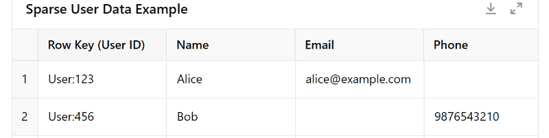
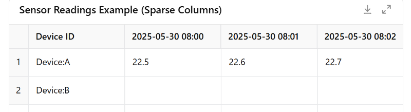
Wide-column stores are great at handling this kind of uneven, dynamic data. They were originally inspired by Google’s Bigtable.

For example, imagine a table of sensor devices where each row is a device ID, and each column stores a reading for a specific timestamp. Some devices might send data every minute (creating thousands of columns), while others send data only once a day. This would be very difficult to manage in a relational database, but wide-column databases handle it efficiently and naturally.

7.2 When to Use It

Wide-column stores are best for big data and high scalability scenarios where the data is large, possibly sparse, and you need to distribute it across many servers. Use cases include:

Time-Series and IoT Data: Storing events or sensor readings. Each device or metric type can be a row, and new readings just create new columns (often grouped into families by time). This allows quick retrieval of a series of readings by row (device) and a time range (since columns can be sorted by key which could be a timestamp). Indeed, some time-series solutions are built on wide-column databases.
Analytical Data (Bigtable style): Google’s original Bigtable (a wide-column DB) was used for things like indexing the web. If you have datasets where each item could have an enormous number of attributes or versions, a wide-column schema could fit. For instance, wide-column databases are used in analytics platforms and data warehousing for storing user events, logs, or aggregated counters, because they can scale out and handle high write rates.
High Write Throughput, Event Logging: Applications that need to log millions of events per second (e.g. click streams, telemetry data) often use wide-column stores (like Cassandra) because they are optimized for fast writes across distributed nodes. The flexible schema means you can just add columns for new event types or attributes without downtime.
Sparse Data with Variable Attributes: Any scenario where different records naturally have very different attributes. For example, consider a large product catalog where products share some core fields but also have many category-specific attributes — one way is a document DB, but another is a wide-column store where each product is a row and you add columns for each attribute that applies. If a new attribute comes along (say a new spec for electronics), you can just add that column to the few relevant rows, without altering a global schema.
Geo-distributed Applications: Some wide-column databases (like Cassandra) are designed to replicate data across multiple data centers easily, making them good for applications that need high availability across regions. The eventual consistency model with tunable consistency fits cases where uptime and partition tolerance are prioritized (e.g., global services that must not go down, even if it means some replicas might lag slightly).

In summary, use a wide-column store when you need the scalability of a key-value store but also want some structure grouping (column families), and when your data doesn’t fit neatly into a fixed schema.

7.3 Key Design Considerations

Data Model and Query Patterns: Designing a schema in a wide-column store is often done query-first. You don’t normalize as in SQL; instead, you might duplicate or pre-compute data to serve your queries efficiently. For example, if you need to fetch a user’s most recent events, you might create a row per user and use column names that sort by time so you can slice the last N columns quickly. Think about your primary access patterns and model the table to optimize those (because querying anything that isn’t designed into the row/column key can be difficult or require full scans).
Partition Keys: The row key (often called partition key) is critical — it determines how data is distributed across the cluster. Choose a key that ensures data is evenly spread. For example, if you use “sensor_id” as the partition key, but one sensor generates 100x more data than others, that one will be a hotspot on one node. Sometimes composite keys or adding a hash/prefix to keys is used to balance load.
Column Family Grouping: Group related columns into families to optimize reads. Columns in the same family are stored together on disk, so reading a subset of columns that are in the same family is efficient. For instance, you might keep all personal info columns in one family and all event count columns in another if you rarely need both at once.
Eventual Consistency and Replication: Wide-column databases (like Cassandra) often default to eventual consistency for distributed writes. You can usually tune the consistency level (e.g., require a write to be confirmed by all replicas vs just a quorum). For critical data, you might up the consistency level at the cost of latency. Also, understand the CAP trade-off — these systems are typically AP (Available and Partition-tolerant) in CAP theorem terms, meaning they may sacrifice immediate consistency. If your application can handle reading slightly stale data during partitions, this is fine; if not, you may need to configure stronger consistency or consider a different DB.
Batch Operations and Compaction: Wide-column stores often encourage batched writes (to amortize overhead). Also, they use log-structured storage under the hood — data is written append-only and then periodically compacted. As a result, performance can be impacted during heavy compaction periods. Monitoring and configuring compaction strategy (size-tiered vs leveled in Cassandra, for example) can be important for performance tuning.
Secondary Indexes: Some wide-column databases provide secondary indexes, but they are usually limited in capability and performance compared to relational DB indexes. In Cassandra, for example, secondary indexes are not recommended for high-cardinality fields. Instead, you might maintain your own index table (another table that maps from a value to the primary key of the main table). Designing those manually is often part of schema design in wide-column models.
Handling of Very Wide Rows: It’s possible (even common) to have rows with millions of columns. While the systems are built for this, extremely wide rows can still pose challenges (e.g., a query that tries to read an entire wide row could time out or OOM if not careful). You might want to break very large logical rows into multiple physical rows (shard by a part of the key like time interval) to avoid any single row from becoming too unwieldy.

7.4 Popular Databases

Apache Cassandra — A highly popular wide-column store, originally developed at Facebook. It’s known for its ability to handle large volumes of writes and its masterless, peer-to-peer architecture that offers no single point of failure.
Apache HBase — An open-source wide-column database that runs on top of Hadoop’s HDFS (inspired directly by Google’s Bigtable). Often used in big data contexts where Hadoop is in play, for example storing time-series or as a backend for Apache Phoenix (an SQL layer).
ScyllaDB — A modern reimplementation of Cassandra in C++ designed for high performance. It offers the wide-column data model and Cassandra compatibility but aims for lower latencies by utilizing resources more efficiently.
Google Cloud Bigtable — Google’s managed wide-column database service (the original Bigtable design). It’s used under the hood in many Google services and available for use on GCP for workloads that need massive scale (e.g., analytics, IoT).
Azure Cosmos DB (Cassandra API) — Azure’s Cosmos DB can emulate a Cassandra wide-column database. This provides a managed, globally distributed option for Cassandra users (with the benefit of Cosmos DB’s turnkey global replication and scaling).

8. Time-Series Databases

8.1 What It Is

A time-series database (TSDB) is specialized for storing time-stamped data, i.e. sequences of values or events indexed by time. The fundamental unit is typically a measurement or event along with a timestamp (and often tags or metadata). Time-series data is everywhere: think of temperature readings captured every minute, stock prices every second, or server CPU usage over time. A TSDB optimizes storage and queries for this kind of data. It often uses compression techniques that take advantage of the fact that consecutive time values or sensor readings are related or don’t change drastically. For example, instead of storing every timestamp in full, it might store a base timestamp for a block of data and deltas for each point. Queries in a TSDB are usually about ranges of time (“give me the last hour of data for sensor X”) or aggregates over time (“compute hourly average over the last week”). These databases make such queries fast by treating time as a primary index. In a sense, a TSDB can be viewed as a hybrid of a key-value store (with the key being something like [metric, timestamp]) and an analytics engine for time-based aggregations.

8.2 When to Use It

Choose a time-series database when your data is predominantly time-indexed and you plan to do a lot of time-based queries or analytics. Common use cases:

Monitoring and DevOps Metrics: Storing infrastructure and application metrics — CPU, memory, request rates, error counts, etc. Tools for monitoring (like Prometheus, Graphite, InfluxDB) are time-series databases under the hood, allowing you to track and graph these over time. For example, to investigate an outage, you might query a TSDB for CPU and memory usage of your servers over the last 24 hours.
IoT and Sensor Data: Any scenario with periodic measurements. Environmental sensors (temperature, humidity), industrial machine readings, smart home device data, etc., all produce continuous streams of time-stamped data. TSDBs are optimized to ingest these at high write rates and allow queries like “what was the reading on sensor X at time Y” or “show me trends and anomalies over time ranges”.
Finance — Ticks and Trading Data: Storing price tick data for stocks, cryptocurrencies, or trading volumes. Time-series databases (or similar structures) can efficiently store millions of price points and let analysts query historical prices or compute moving averages. (In ultra-low-latency trading, specialized systems like kdb+ are used, which is a kind of time-series columnar DB).
Scientific and Medical Data: Experiments or monitoring that record values over time, like telemetry from a spacecraft, or patient vital signs streaming in a hospital. A TSDB can store these and handle queries for trends or threshold breaches (e.g. find when a reading went above a certain value).
Usage Analytics: Time-stamped events like page views, clicks, or transactions can be stored in a TSDB (though often they might also be stored in analytical databases or big data systems). If you want quick aggregations by time (say, requests per minute), a TSDB structure can be very handy.

In summary, if your data naturally comes in an ever-growing time-indexed sequence and you rarely (or never) update past data points (you mostly add new ones), and you want to efficiently query ranges or do rollups (min, max, avg over intervals), a time-series database is the right tool.

8.3 Key Design Considerations

Data Retention and Downsampling: Time-series data can grow without bound. A key strategy is retention policies — decide how long to keep raw data. For example, keep 1-second granularity data for one week, then automatically downsample or delete older data (perhaps storing only 1-minute averages for anything older). Many TSDBs support automatic retention and downsampling. Plan what level of historical detail you truly need, as keeping everything forever can become expensive.
Compression and Storage: TSDBs often use compression tailored to time-series (for example, Facebook’s Gorilla compression for metrics). This means you can often store a lot more data in the same space compared to storing timestamps and values in a general database. Check the compression and ensure your data characteristics (frequency, typical value changes) align with it. Sometimes you might choose data types (float vs integer) or value resolutions to maximize compression.
High Ingestion Rates: Time-series use cases often involve ingesting streams of data from many sources. TSDBs are optimized for high write rates, but you should consider how to batch or stream inserts efficiently. If using a system like InfluxDB or TimescaleDB, for example, using their bulk write protocols or JSON line formats can greatly improve throughput versus individual inserts.
Indexing and Query Patterns: Typically, the primary index is time. Many TSDBs partition data by time internally (like chunks per hour or day). Still, you often have tags or secondary dimensions (e.g. server ID, location, metric type). TSDBs like InfluxDB or Prometheus allow tagging data points, and you can query something like WHERE location='east' AND sensor_type='temperature' AND time > now()-1h. Under the hood, the DB must manage those indexes. Be mindful of cardinality: if you create millions of unique tag values (like using a high-cardinality field as a tag), it can bloat memory and index. A common consideration is to limit high-cardinality tags (e.g., don’t tag each request with a unique ID; tag by broader categories like service name or data center).
Out-of-Order Data: In some systems (especially IoT), data might not arrive in perfect time order — e.g. a device goes offline and later sends a batch of readings. TSDBs usually handle out-of-order inserts, but performance can degrade if too much comes out of order (since they ideally write append-only in time). Check how your DB handles it — some might drop very old out-of-order data or require special config. If you expect a lot of late data, you might need to increase the window for out-of-order writes or use a system that handles reordering well.
Aggregation and Query Functions: Time-series queries often involve aggregation (avg, sum, min, max) over time windows, or transformations like rate of change. Many TSDBs provide these as query functions or in their query language (e.g., InfluxQL, PromQL, Timescale SQL extensions). Make use of these built-ins for efficiency rather than pulling raw data and aggregating in your application. Also consider setting up continuous queries or materialized views if you frequently need certain rollups (like daily summaries).
Integration with Visualization/Monitoring Tools: A lot of value from TSDBs comes when combined with visualization or alerting (like using Grafana dashboards or setting alerts on thresholds). Ensure the TSDB you choose integrates well with your monitoring/alerting stack. For example, Prometheus is often paired with Grafana for dashboards and Alertmanager for alerts. The ease of use of these tools might influence your choice of TSDB.

8.4 Popular Databases

InfluxDB — A popular open-source time-series database with its own SQL-like query language (InfluxQL) and a newer Flux language. Often used for DevOps monitoring, IoT, and application metrics.
TimescaleDB — An extension built on PostgreSQL that turns it into a time-series database. It allows you to use SQL (including complex joins) on time-series data, and it automatically partitions data by time for you. Good for those who want both time-series performance and the familiarity of SQL.
Prometheus — An open-source monitoring system and TSDB, part of the Cloud Native Computing Foundation. It’s designed for monitoring infrastructure and applications, comes with a powerful query language (PromQL), and is often used for scraping metrics from services. It’s not a general-purpose TSDB for arbitrary apps (more tailored to monitoring use).
OpenTSDB — A distributed time-series database built on top of HBase (wide-column store). It was one of the earlier big-data TSDBs and can handle very high write rates by leveraging HBase’s scalability. Used in some large enterprises for infrastructure metrics.
Graphite — An older time-series system focused on storing metrics and generating graphs. It’s file-based (whisper DB) and not as scalable as newer solutions, but it introduced concepts that influenced others. Often replaced by more modern systems now, but still used in some legacy setups or smaller deployments.
(There are many others, like VictoriaMetrics, Apache IoTDB, AWS Timestream, etc., but the above are some of the well-known ones.)

9. Blob Storage (Binary Large Object Stores)

9.1 What It Is

A blob store isn’t a traditional “database” for structured queries, but rather a system optimized for storing and retrieving large binary files or unstructured data. Blob stands for Binary Large Object. Blob storage is essentially a distributed file storage where you can put or get files (documents, images, videos, backups, etc.) identified by a key or path. The storage system doesn’t attempt to understand the content of the files — it just treats them as opaque streams of bytes. You typically interact with a blob store via simple commands: put (to upload a file with a key), get (to retrieve it by key), delete, etc. Under the hood, blob stores handle replication and distribution of data to be fault-tolerant and scalable. For example, if a user uploads a profile picture or a PDF document, it makes sense to store it in a blob store and save only a reference (URL or key) in a traditional database. The blob system will keep the file safe and accessible. One key aspect: blob stores usually use the file path or object key as the index — that’s how you locate your data. They do not index the content of the file (unless you add extra services on top). So if you need to find something inside a lot of blob files, you’d have to scan through them or use a search system. Blob storage excels at just holding large files reliably and cheaply.

9.2 When to Use It

Use blob storage whenever you need to store large, unstructured files or large binary data, especially if the files need to be accessed or downloaded by different systems or users. Scenarios include:

User-Generated Content: Photos, videos, audio uploads, attachments — any user file uploads in an application. For example, a photo-sharing app will use blob storage to save the photos and thumbnails. The app’s database might store metadata (caption, owner, etc.) and a link to the blob storage where the image bytes reside.
Backups and Archives: Storing database backups, log archives, or any infrequently accessed data. Blob stores are usually much cheaper per GB and can scale to petabytes, so they’re ideal for archiving. For instance, a company might dump daily logs or analytics data as files into blob storage for later processing.
Media Streaming: Videos and audio files for streaming services are kept in blob storage. The service can then pull from the blob store to stream to users. Blob stores often integrate with CDNs (Content Delivery Networks) for distributing this content globally.
Big Data Lakes: Often, organizations build data lakes where raw data (CSV files, JSON dumps, images, etc.) are all stored in a blob store (like an object storage service). Tools like Hadoop or Spark can then directly read from the blob storage (which acts like a giant distributed file system) for processing.
Documents and Reports: In enterprise apps, if you generate PDF reports, invoices, or store scanned documents, those binary files go into a blob store, referenced by a key in a database.
Machine Learning Data: Large training datasets (images, video clips, sensor recordings) are kept in blob storage because of volume. ML pipelines fetch the needed objects from the blob store for training models.

In essence, use blob storage any time you have files or large chunks of data that don’t need to be queried by their internal structure. It provides a cheap, scalable repository for such blobs, leaving your databases free to handle the metadata and structured info.

9.3 Key Design Considerations

No Content Querying: As noted, you can’t query within the file via the blob store. If you need to find files by some attribute, you must maintain that metadata externally (e.g., in a relational DB or search index). For instance, if you have millions of PDF documents and you want to search their contents, you’d need a full-text search system indexing those PDFs; the blob store alone can’t do that. Plan to store and index metadata like file type, upload date, tags, or user associations in a separate database for querying purposes.
Consistency and Durability: Blob storage systems (like cloud object stores) are typically designed for high durability — meaning multiple copies or erasure-coded shards of your file are stored so that hardware failures don’t lose data. Most provide eventual consistency for listing or reading recently written objects. (Notably, Amazon S3 now offers strong read-after-write consistency for new puts, but historically object stores were eventually consistent on updates/deletes). If your use case involves reading an object immediately after write, be aware of the consistency guarantees. In most cases it’s a non-issue, but it’s good to know the specifics of your blob store (especially if you overwrite or delete objects frequently).
Performance and Access Patterns: Blob stores are optimized for throughput rather than low latency. Retrieving a large file might take some time as it streams from disk or across the network. They usually handle range requests (so a video player can fetch a chunk of a video file, for example). If you have an application that needs to frequently access small pieces of many files, a blob store might be slower than a database that can index and cache those pieces. In such cases, consider if you should break files into smaller pieces or use a different storage approach. Also, pay attention to concurrency limits — e.g., how many requests per second you can make per bucket or per account, and use CDNs or caching layers if you will serve hot objects to many users.
Cost Management: One of the big reasons to use blob storage is cost — storage per GB is usually much cheaper than keeping data in databases or local servers. But costs can add up with large scale, and cloud providers charge not just for storage but also for operations (each read/write request, data egress bandwidth, etc.). Design your system to minimize unnecessary data transfer (use caching for popular objects, compress files if appropriate, and delete data you no longer need). Also consider lifecycle rules — for example, automatically move data to a colder storage class (cheaper storage, but slower access) if it hasn’t been accessed in 90 days, to save cost. Many blob stores offer tiered storage classes (like AWS S3 Standard vs Glacier).
Security and Access Control: Store sensitive files securely. Blob stores typically allow setting permissions on buckets or individual objects. Use features like pre-signed URLs or access tokens to control who can download a file. If you’re designing multi-tenant storage, avoid putting all user files in one flat namespace without proper access control. Also consider encryption — most blob stores can encrypt data at rest, and you might want to encrypt at the application level for extra security.
Multipart and Large Files: If you deal with very large files (hundreds of GB or more), blob stores usually support multipart uploads — uploading the file in parallel chunks. For downloading, similarly, clients can fetch ranges in parallel. Use these capabilities to speed up transfer of giant files. Also, some stores have a maximum single-object size (like 5TB for S3); if you need beyond that, you’d have to split the data.
Metadata on Objects: Blob stores often let you store a small amount of metadata along with each object (like content type, cache control headers, or custom key-value metadata). Use this for things like setting the MIME type (so browsers know how to handle it) or tagging the object with something like an ID or type that you might use in code. But remember, these metadata are not indexed for search; they are only retrievable if you know the object.

9.4 Popular Databases (Blob/Object Stores)

Amazon S3 — Amazon Simple Storage Service, the archetype of cloud object storage. It’s highly durable (11 nines of durability) and scalable. Many applications integrate with S3 for storing files.
Azure Blob Storage — Microsoft Azure’s blob storage service. Similar use cases to S3, used in Azure cloud deployments for any file storage needs (from media content to VM disk snapshots).
Google Cloud Storage (GCS) — Google Cloud’s object storage offering. Often used for data lakes, ML datasets, and web asset storage in GCP.
MinIO — An open-source object storage server you can self-host. It’s S3-compatible, meaning it offers the same API. Good for on-premises setups or edge where you need S3-like storage functionality.
Ceph (RADOS Gateway) — Ceph is an open-source distributed storage system; its RADOS Gateway provides an object storage interface (also S3-compatible). Used in many private cloud or OpenStack environments for object storage needs.
(These systems are typically accessed via HTTP APIs or SDKs, not via SQL. They are sometimes called “datastores” rather than databases, but they are a crucial part of the data storage landscape.)

10. Spatial Databases

10.1 What It Is

Spatial databases are databases that are optimized to store and query geospatial data — that is, data representing objects or locations on earth (or any geometric space). They introduce special data types for geometry: points (a single coordinate like a latitude/longitude), lines (e.g. a road or river), polygons (e.g. a country’s boundaries or a lake), etc. What makes a database “spatial” is not just storing these as data, but the ability to perform spatial queries using these types. For example, a spatial database can answer questions like “Which points fall within this polygon?” or “What is the distance between these two points?” or “Find all records whose location is within 5 kilometers of the user’s location.” These databases use spatial indexes (like R-trees, Quad-trees, or Geohash-based indexes) to speed up such queriespostgis.net. A common approach is an R-tree index, which groups nearby objects so the database can quickly eliminate large irrelevant areas when searching. An everyday example: if you have a database of store locations (each a point with latitude and longitude), a spatial database would allow you to efficiently find “the 10 stores closest to me” or “all stores within California” with a single query. Essentially, spatial databases extend the SQL language with geometric functions and use the principles of computational geometry under the hood to answer location-based questions.

10.2 When to Use It

Use a spatial database if your application deals heavily with location-based data or geometry and you need to run queries based on spatial relationships. Examples:

Location-Based Services: If you’re building features like “find nearby restaurants,” “show me all users in this region,” or mapping applications (e.g. Uber/Lyft finding drivers near riders), a spatial DB is a natural fit. It will handle the math of great-circle distance and area calculations for you.
Geographic Information Systems (GIS): Government or environmental data, such as maps of roads, land use, water bodies, etc., are managed in spatial databases. GIS analysts might store thousands of polygons representing city boundaries, zoning districts, flood zones, etc., and query things like “which homes are in flood zone A” or “what area of forest was affected by this fire polygon.”
Asset Tracking: Storing moving object data like vehicle GPS coordinates over time. A spatial DB can store the paths as lines or sequences of points and let you query, for example, which vehicles were within a certain area during a time window.
Spatial Analytics: If you need to do analysis like clustering of points (finding hotspots), checking coverage (e.g. do my store locations cover all regions within 10 miles?), or spatial joins (like pairing each customer to the nearest store), spatial extensions make these tasks much easier with SQL functions.
CAD/Architecture/Engineering Data: Spatial DBs can also store geometric shapes in 2D/3D for use in technical fields, supporting queries like intersection, containment, and proximity which might be useful in planning or design applications.
Games/AR: In augmented reality or games with geolocation (e.g. Pokémon Go), a spatial database could be used to manage game objects and efficiently find what’s near a player’s location.

In short, if you find yourself needing to query data by “where” questions (within, nearby, intersection, distance), a spatial database will be very beneficial.

10.3 Key Design Considerations

Spatial Indexing: The effectiveness of a spatial query often comes down to the spatial index. Make sure to create indexes on your geometry columns (most spatial DBs don’t automatically index a geometry column unless you ask). For example, in PostGIS (PostgreSQL’s spatial extension), you’d create a GIST or SP-GIST index on the geometry column. This dramatically improves query speed for location-based queries, as it prunes the search space using bounding boxespostgis.net. Without an index, spatial queries will fall back to brute force checking of every geometry, which is very slow when you have lots of data.
Coordinate Systems (Projections): Geospatial data can be represented in different coordinate systems (latitude/longitude is one, but there are many map projections). Spatial databases typically allow you to specify an SRID (Spatial Reference ID) for your data, which defines the coordinate system. It’s important to be consistent — data has to be compared/queried in the same coordinate system or be transformed. If you store everything in lat/long (WGS84), functions that calculate distance need to account for the earth’s curvature (great-circle distance). Some spatial DBs provide functions for geodetic (curved surface) calculations vs planar calculations. Choose what makes sense (for small areas, planar might be fine; for global, use geodetic functions).
Query Accuracy vs Performance: Operations like ST_DWithin (within a distance) or ST_Contains (one geometry contains another) have to balance accuracy and speed. For example, calculating exact distance on an ellipsoid Earth model is expensive; some systems approximate or require you to use a geography type vs geometry type for different behaviors. You might decide to use a faster approximate index for initial filtering (e.g. bounding box check) then a precise calculation for final filtering. Be aware of these details if high precision is needed (like in legal land parcel definitions) versus if an approximation is acceptable (like a rough search radius).
Data Volume and Simplification: Spatial data, especially polygons and lines, can be very detailed (think of a country border with thousands of points). Complex geometries can slow down operations. It’s often useful to store a simplified version of geometry for certain queries or zoom levels. For example, you might have a highly detailed coastline polygon for accurate analysis, but for a broad “what counties intersect this area” query or for rendering on a small map, you could use a simplified geometry. Some databases or GIS tools have functions to simplify geometries (reduce vertex count) which can speed up computations.
Update Patterns: If your spatial data is mostly static (like maps), query performance is the main focus. If you have dynamic spatial data (like moving vehicles updated every few seconds), consider the cost of constantly updating spatial indexes. Some spatial databases handle this well, but it could be heavy if you’re updating thousands of geometries per second. In cases of heavy writes, you might need to partition data or use simpler spatial data types (like points are simpler than complex polygons) for dynamic data.
Spatial Joins: One of the most powerful features is joining two spatial datasets by location (e.g., join customers to regions to see which region each customer falls in). These can be expensive operations if datasets are large. Ensure indexes exist on at least one side of the join and consider tiling or partitioning strategies if data is extremely large (e.g. dividing space into regions and only joining relevant regions to limit comparisons). Some systems allow parallel spatial joins if data is partitioned by space.
Use of Extensions vs Built-in: Many relational DBs have spatial extensions (PostGIS for PostgreSQL, SpatiaLite for SQLite, Oracle Spatial, MS SQL Server has geography types, etc.). Using them means your app can query spatially using SQL. Alternatively, specialized spatial databases or GIS might offer more features but could be separate from your main DB. Weigh the convenience of having everything in one database vs possibly using a dedicated spatial engine (for example, some people export data to something like an ElasticSearch with geo-capabilities for certain location queries, or use a cloud service like Google BigQuery GIS). For most cases, an extension like PostGIS is extremely powerful and full-featured.

10.4 Popular Databases

PostGIS (PostgreSQL) — An extension to PostgreSQL that turns it into probably the most feature-rich open-source spatial database. It supports both geometry (planar) and geography (curved earth) types, and hundreds of functions for every spatial operation (distance, area, buffer, intersections, you name it). This is a go-to for many GIS applications and is widely used in mapping communities.
Oracle Spatial and Graph — Oracle’s enterprise database includes spatial capabilities (and graph). It’s used by many large organizations for GIS and spatial analytics, with support for advanced features and coordinate systems.
Microsoft SQL Server (Spatial) — SQL Server has geometry and geography types built-in, and supports spatial indexes and queries via T-SQL. It’s not as exhaustive in functions as PostGIS, but it covers most common needs (distance, within, intersects, etc.) and is convenient for those in the MS ecosystem.
Spatialite (SQLite extension) — An extension for the file-based SQLite database that adds spatial SQL support. It’s useful for lightweight applications or mobile apps that need a local spatial database.
Neo4j with Spatial (and others) — There are graph and NoSQL databases that have geospatial indexing as well. For instance, MongoDB has geospatial index types for simple “near” queries on points. ElasticSearch/OpenSearch can index geo points or shapes for geospatial search. These aren’t full-fledged spatial databases in the GIS sense, but if your needs are simple (mostly point-in-radius queries), they can be an alternative. For full GIS workloads, a specialized spatial RDBMS like PostGIS is usually the top choice.

Each database category above has its unique strengths and ideal use cases. In practice, modern applications often use a combination of these systems side by side — for example, a relational database for core business data, a document database for logging or user-generated content, a search engine for text queries, and a blob store for files. Knowing the role each plays will help you choose the right database (or databases) to make your system efficient, scalable, and maintainable. Use this guide as a starting point for evaluating what fits your project’s needs, and don’t be afraid to adopt a polyglot approach if one size doesn’t fit all. By leveraging the proper data store for each task, you’ll achieve better performance and flexibility in the long run.

Choosing the Right Database: Types, Use Cases, and Design Considerations

Table of contents