Step-by-Step Guide On Implementing Neural Networks From Scratch - Part 2

In my previous article, we’ve learnt about neural networks, the intuition and the theory behind them. (Although I glossed over forward and backward propagation, don’t worry we’ll go over them clearly today!)

In this article, I’m going to go through the math behind neural networks. Yep, we’ll need just one more article to finish neural networks.

So first, let’s recall our network and outline the steps we need to follow. This will make it easier for us to develop our network throughout the chapter without having to go back to the previous article. (Unless you’re binge-reading this, in which case you’ll remember everything, so no worries.)

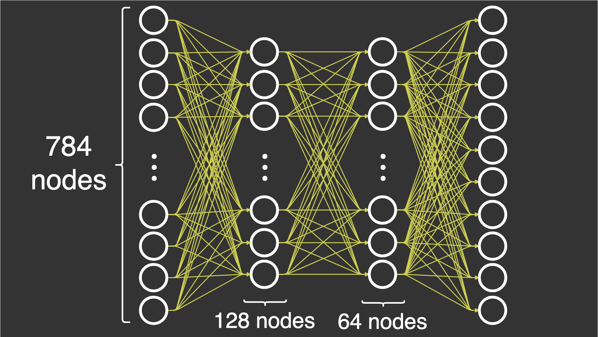
So we’ve decide on our dataset to be the famous MNIST dataset. It’s a dataset containing almost 60,000 examples of 28×28 grayscale images of handwritten digits. We’ve also decided to create a 4-layer network (including input and output) consisting of the input layer, 2 hidden layers with 128 and 64 neurons respectively, and the output layer consisting of 10 neurons. (Because I was too lazy to edit the picture below for another set of number of neurons in each layer)

Now our first task is to create our dataset and prepare to send it one by one into the network.

(Ah btw I’m gonna use google colab for the project so I will be importing the dataset from keras. Yes, I remember what I said, “from scratch”. I’m only gonna import the dataset, don’t worry)

import numpy as np
from tensorflow.keras.datasets import mnist

See? there we go. We’re importing numpy and the dataset that’s it.

Now, we will be doing something called preprocessing, this is where the input we need to send to the network is modified for performance and other considerations. We won’t be going too much into detail because preprocessing is a story for another time.

# Load MNIST data
(x_train, y_train), (x_test, y_test) = mnist.load_data()

# Normalize and reshape the input data
x_train = x_train.reshape(-1, 28 * 28).astype('float32') / 255.0
x_test = x_test.reshape(-1, 28 * 28).astype('float32') / 255.0
x_train, x_test = x_train.T, x_test.T  # Transpose for easier manipulation

This is what we’ve done here

• We loaded the dataset using the load_data() method

• We then normalized the dataset, what you need to know here is that if you try to observe the dataset, we get 28 × 28 matrix values for each test case, so we will be transforming that into 784 columns of single row examples. The -1 indicates that “I’m too lazy to figure your actual shape so figure it out on your own, I just want 784 columns” (Pretty convenient, yeah?)

• Also another thing is we get values between 0 - 255 in the values, so we’re dividing by 255 to keep the values between 0 and 1 (Note that diving an entire dataset by a constant does not change the relative relationship with other values in the dataset.

• And finally we transpose the dataset by using the .T (basically shifting rows to columns and vice versa)

Now that we’re done with preprocessing, let’s talk about what we need to make our computations easier in the future.

We need to decide on our activation function before we create throw the inputs into the layer. This topic was briefly mentioned in the previous article but now, we’ll be going into a full deep-dive on activation functions.

Activation Function

Let’s step back for a bit and look at our list of tasks now that we’ve normalized and prepared our inputs. Our next step is to send these inputs to the next layer, where they are multiplied by certain weights and added to a bias to obtain a new number. That new number will then be sent to the next layer. Let’s pause here for a moment.

Our next step is to send these inputs to the next layer, where they are multiplied with a certain weight and added to a bias to obtain a new number

Does that sound familiar? Yes, this is exactly what a linear model does. So this activation function is what adds complexity to our linear model to turn it into a neural network that can solve complex problems. You need complexity to solve complexity, sounds nice eh?

Don’t worry, activation function itself isn’t complex, it just adds complexity to the network. Let’s see how:

The activation function constraints the output range of a neuron to a specific interval (e.g., between 0 and 1). This is the additional layer of complexity we’re talking about, to explain it in simpler terms, what an activation function does is takes an input number and spits out an output number which is between the specified range. (like between 0 and 1)

How does it do this? Activation functions are nothing more than mathematical formulas. Here are a few famous activation functions and their formulas

Sigmoid

$$\sigma(x) = \frac{1}{1 + \exp^{-x}}$$

The output range for sigmoid is between 0 and 1. To learn more about sigmoid, read this.

Tanh ( Hyperbolic tangent )

$$tanh(x) = \frac{e^x - e^{-x}}{e^{x}+e^{-x}}$$

The output range for tanh is between -1 and 1.

ReLU

$$ReLU(x) = max(0, x)$$

The output range for ReLU is [0, ∞)

To learn about more activation functions read here.

Congratulations, now you know everything you need to know about a single neuron.

And a cool detail here, neural network is a combination of linear regression and logistic regression. (not completely, but yeah mostly since activation function is not strictly logistic)

$$\displaylines{ Z = WX + b \quad *linear\;part \\ A = \sigma(Z) \quad *activation\;part }$$

Let’s define all the functions that we need in our neural network as we go.

def ReLU(Z):
    return np.maximum(Z, 0)

That’s the literal definition of ReLU we’ve defined above.

Forward Propagation

Now, let’s actually dry run our network with the inputs to discover what we need next (we’re reinventing neural networks after all, so discover is appropriate here)

By dry-running, I mean we’re going to observe how our input changes as it passes through the layers, and how the shape of our data evolves over time.

Let’s separate our neuron’s operations into 2 parts, linear and activation. The result we get from the linear part will be represented as Z and the result from activation function will be represented as A. That’s the convention I’ll be using from now and the one I used before. Please keep that in mind.

Also, we will be using a superscript to identify which layer a value belongs to, for example:

$$Z^{[l]}\quad implies\; that \; this \; Z \; belongs \; to\; the\; layer\; number\; l$$

Now that we know of the convention, let’s get back to dry running

$$\displaylines{ Z^{[1]} = W^{[1]}X + b^{[1]} \\ }$$

Our W[1] here is of shape (128 × 784). Why?

Here’s a simple rule of thumb you can follow for weights, if the shape is of (m x n) you can blindly say that m is equal to the number of neurons in the present layer (Note that, we are not calculating individually but the layer as a whole, so Z[1] here contains all values of neurons from layer 1) and n is equal to the number of neurons in the previous layer.

And the shape of b[1] is (128, 1). As it is a scalar value (a single bias per neuron) that we will add in each neuron it is in the shape of the number of neurons in that layer.

So the shape of Z[1] is

$$\displaylines{ Z^{[1]} = W^{[1]}X + b^{[1]} \\ Z_{?} = W_{(128\times784)}^{[1]}X_{(784\times1)}^{[1]}+b_{(128\times1)}^{[1]} \\ Z_{?} = [WX]{(128\times1)}^{[1]}+b{(128\times1)}^{[1]} \\ Z_{(128\times1)} = [WX + b]_{(128\times1)}^{[1]} }$$

Now, we will send this calculated linear part into our Activation function, we’re going to choose ReLU for this layer

$$A_{(128\times1)}^{[1]} = ReLU(Z_{(128\times1)}^{[1]})$$

We’re done with computing the first layer, now we need to send this output from activation function as input to the next layer, that’s what the network is all about, neurons from previous layer conversations with neurons in the next layer.

And, now let’s define the shape of W[2], as stated by our rule of thumb before it’s shape is going to be (64 × 128)

$$\displaylines { Z_{(?)}^{[2]} = W_{(64\times128)}^{[2]}A_{(128\times1)}^{[1]} + b_{(64\times1)}^{[2]} \\ Z_{(?)}^{[2]} = [WA]{(64\times1)}^{[2]}+ b{(64\times1)}^{[2]} \\ Z_{(64\times1)}^{[2]} = [WA + b]_{(64\times1)}^{[2]} }$$

I’m sure you know what’s going to come now. Yes, activation function. (We’ll be using ReLU in this layer as well)

$$A_{(64\times1)}^{[2]} = ReLU(Z_{(64\times1)}^{[2]})$$

Now comes the last layer, the output layer, which also has linear part and activation part. Here’s the change, for the activation part in the output layer we will be using softmax function.

What is softmax function you ask? Let’s get to it after the linear part. One step at a time people.

The shape of W for this layer is, as you’ve guessed, (10 × 64). Wow, you’re getting good at this!

$$\displaylines{ Z_{(?)}^{[3]} = W_{(10\times64)}^{[3]}A_{(64\times1)}^{[2]} + b_{(10\times1)}^{[3]} \\ Z_{(?)}^{[3]} = [WA]{(10\times1)}^{[3]}+ b{(10\times1)}^{[3]} \\ Z_{(10\times1)}^{[3]} = [WA + b]_{(10\times1)}^{[2]} }$$

Great! Now, we can finally move on to the softmax part.

Softmax

Why softmax? Before we understand that, let’s look at our output for a given input of (784×1). The output shape is (10×1). A vector / single column matrix / single row matrix, basically a list of 10 numbers. And there’s one thing about this vector that’s special, it’s that it only contains either 0 or 1. Additionally, there’s only a single 1 and all other 9 values are 0s.

Why?

Think of our problem set, it’s a dataset containing almost 60,000 examples of 28×28 handwritten digits. Yes, handwritten digits, single digits, and these digits can only be from 0 to 9. Now you understand where the shape (10×1) comes from? It’s a vector of size 10, where the correct digit is 1 and all other options are 0. I’ll let you take a while to think over that.

(E.g., if the input is a picture of 2, then y will be equal to [0, 0, 1, 0, 0, 0, 0, 0, 0, 0])

Now then, you might be asking me “sure, but what does that have to do with softmax?”. Let me get to it now, the softmax function (not sure why they names it that, but whatever) takes a whole vector and changes all the values in it with respect to the other values, yes you heard that right, and I think that’s the most simplest explanation someone can give. Basically what it does is, it takes let’s say 5th number in the vector and compares (not really, but we’ll get to that) it with other numbers and reassigns this 5th number to a new number.

What does it reassign the number to? That’s the main part. Softmax works with probabilities, it takes all the values and reassigns values such that, the sum of all the numbers in the vector will equal to one. So what this essentially does is, it assigns the highest probability to let’s say 5th position again, implying that 5 is the expected output.

There’s 3 things to remember for softmax.

• After softmax, all the numbers in vector will be constrained to values between 0 and 1.

• The sum of all the numbers in the said vector will be equal to 1.

• The index place of the number with the possibility of being the answer will be assigned the highest probability.

Now that you know what softmax is, and why we used it in the output layer, let’s get back to business.

$$\displaylines{ A_{(10\times1)}^{[3]} = softmax(Z_{(10\times1)}^{[3]}) \\ softmax(X) = \frac{e^{x_i}}{\sum_{i = 1}^{n}e^{x_i}} }$$

This A[3] also happens to be our Y_pred.

That is it for forward propagation of this network.

Backward Propagation

Backward propagation. The dreaded topic. Yes, it’s a dreaded topic for most, but don’t worry, I’ll make it as simple as possible.

So what is back propagation anyway? As its name suggests, we are now going to propagate backward. But why backward? Let’s try to think about this intuitively, you’ve just created a model where you send data forward starting from input layer until the output layer. So do you think our predictions are somehow magically correct because we just sent them through a few hidden layers using some complicated math? (You’re prolly not, but this just adds some spice, so I’ll leave it that way)

Anyways, since we hypothetically initialized (not yet in code) our weights randomly (refer to previous chapter) the answers we get from our forward propagation are just pure random guesses to say the least. And that is why we need to calculate the error i.e., the difference between the actual output and predicted output. And using that error we need to change our weights, in a way that reduces the said error.

So, how do we do all that? Don’t worry we’ll go over it step by step now.

First, let’s get this straight, when I said “we are now going to propagate backward”, I don’t literally mean going backward, it’s just a metaphor, but in a way, we will compute the errors by going backward in the network layer-by-layer.

Let’s first define our error function.

The error / loss function we’re going to use here is called cross-entropy. It is defined as follows,

$$\displaylines{ L = -\sum_{i=1}^{10}y_ilog(\hat{y_i}) \\ remember,\; \hat{y} = A^{[3]} }$$

This gives us a scalar value.

Now using this loss function, we will calculate how this loss is affected by weights from each layer. The math is what’s flowing backward here. This method, btw, is called the gradient calculation via partial derivation.

Now let’s understand what all we need to calculate. By now, you probably understand that we need to change the weights (Ws) and biases (Bs) to reduce the errors.

We need to change all W3, B3, W2, B2, W1, and B1. And to make our calculations easier, we will start from backward, i.e., W3 and B3.

$$\displaylines{ \frac{\partial{L}}{\partial{W^{[3]}}} = \;? }$$

Don’t worry, I put the question there on purpose, and that is to make you understand what we need to calculate here. Let’s understand, how is L related to W?

L is directly related to A[3] as defined above. And if you look at the previous calculations, A[3] is equal to the softmax(Z[3]), Z[3] is equal to W[3]A[2] + b[3]. Are you getting the hang of this now?

$$\displaylines{ \frac{\partial{L}}{\partial{W^{[3]}}} = \frac{\partial{L}}{\partial{A^{[3]}}}\frac{\partial{A^{[3]}}}{\partial{Z^{[3]}}}\frac{\partial{Z^{[3]}}}{\partial{W^{[3]}}} \\ = [\frac{\partial{L}}{\partial{A^{[3]}}}\frac{\partial{A^{[3]}}}{\partial{Z^{[3]}}} \; is \; simply\; the \; derivative\; of \; softmax\; with\; respect\; to \; A^{[3]}] \\ (Let's \; assume \; that \; value\; is \; equal\; to \; SD \; for \;now.) \\ = [\frac{\partial{Z^{[3]}}}{\partial{W^{[3]}}} = \frac{\partial{(W^{[3]}A^{[2]} + b^{[3]}}}{\partial{W^{[3]}}}] \\ = (SD)A^{[2]} }$$

Let’s compute the value of SD now.

$$\displaylines{ Calculating\; \frac{\partial{A^{[3]}}}{\partial{Z^{[3]}}} \; now \\ \frac{\partial{A^{[3]}}}{\partial{Z^{[3]}}} = \frac{\partial{a_i}}{\partial{z_i}} \\ (ai = \frac{e^{z_i}}{e^{z_i} + e^{z_j} + \sum_{k \ne (i, j)}e^{z_k}}) \\ there \; are\; 2\; cases\; to\; consider\; here\; \\ case\;1: j = i \\ case\;2: j \ne i \\ }$$

For case 1:

$$\displaylines{ Case\;1: j = i \\ \frac{\partial}{\partial{z_i}}(\frac{e^{z_i}}{e^{z_i} + \sum_{k \ne j}{e^{z_k}}}) = \\ We'll\; be\; using\; the\; formula\; \frac{\partial}{\partial{x}}\frac{u}{v} = \frac{v\frac{\partial{u}}{\partial{x}} - u\frac{\partial{v}}{\partial{x}}}{v^2} \\ = \frac{(e^{z_i} + \sum{e^{z_k}})(e^{z_i}) - (e^{z_i})(e^{z_i} + 0)}{(e^{z_i} + \sum{e^{z_k}})^2} \\ = \frac{e^{z_i}\not{e^{z_i}} + e^{z_i}\sum{e^{z_k} - e^{z_i}\not{e^{z_i}}}}{(e^{z_i} + \sum{e^{z_k}})^2} \\ = \frac{e^{z_i}\sum{e^{z_k}}}{(\sum{e^{z_i}})^2} \\ = \frac{e^{z_i}}{\sum{e^{z_i}}} \frac{\sum{e^{z_k}}}{\sum{e^{z_i}}} \\ Note\; that\; \frac{e^{z_i}}{\sum{e^{z_i}}}\; is\; equal\; to\; a_i \; itself! \\ And\; now \; \frac{\sum_{k \ne i}{e^{z_k}}}{\sum{e^{z_i}}} is\; equal\; to\; 1 - a_i \; \\ 1 - \frac{e^{z_i}}{\sum{e^{z_i}}} = 1 - a_i \\ Finally, \\ \frac{\partial}{\partial{z_i}}(\frac{e^{z_i}}{e^{z_i} + \sum_{k \ne j}{e^{z_k}}}) = a_i (1 - a_i) }$$

Now for case 2:

$$\displaylines{ Case\;2: j \ne i \\ \frac{\partial{a_i}}{\partial{z_j}}(\frac{e^{z_i}}{e^{z_i} + e^{z_j} + \sum_{k \ne{i,j}}{e^{z_k}}}) = \\ We'll\; be\; using\; the\; same\; formula\; \frac{\partial}{\partial{x}}\frac{u}{v} = \frac{v\frac{\partial{u}}{\partial{x}} - u\frac{\partial{v}}{\partial{x}}}{v^2} \\ = \frac{(e^{z_i} + e^{z_j} + \sum_{k \ne{i,j}}{e^{z_k}})(0) - (e^{z_i})(e^{z_j} + 0)}{(e^{z_i} + e^{z_j} + \sum_{k \ne{i,j}}{e^{z_k}})^2} \\ = \frac{-e^{z_i}e^{z_j}}{(\sum{e^{z_i}})^2} \\ = -\frac{e^{z_i}}{\sum{e^{z_i}}}\frac{e^{z_j}}{\sum{e^{z_i}}} \\ Note\; that\; \frac{e^{z_i}}{\sum{e^{z_i}}}\; is\; equal\; to\; a_i \; itself! \\ And\; now \; \frac{e^{z_j}}{\sum{e^{z_i}}}\; is\; equal\; to\; a_j \; itself! \\ Finally, \\ \frac{\partial{a_i}}{\partial{z_j}}(\frac{e^{z_i}}{e^{z_i} + e^{z_j} + \sum_{k \ne{i,j}}{e^{z_k}}}) = - a_ia_j }$$

Combining these cases, we can simplify as following:

$$\frac{\partial A^{[3]}}{\partial Z^{[3]}} = \frac{\partial{a_i}}{\partial{z_j}} = \begin{cases} -a_ia_j \quad if\; i \ne j \\ a_i(1 - a_i) \quad if \; i = j \end{cases}$$

Now let’s the other part:

$$\displaylines{ Calculating\; \frac{\partial{L}}{\partial{A^{[3]}}}\; now \\ (Loss)\; L = -\sum_{i=1}^{10}y_ilog(\hat{y_i})\\ remember,\; \hat{y} = A^{[3]} \\ Therefore, \;L = -(y_ilog(a_i) + \sum_{j \ne i}y_jlog(a_j)) }$$

$$\displaylines{ \frac{\partial{L}}{\partial{A^{[3]}}} \frac{\partial{A^{[3]}}}{\partial Z_i } = \frac{\partial{L}}{\partial{Z^{[3]}}} = -\frac{\partial}{\partial z_i}(y_ilog(a_i) + \sum y_klog(a_k)) \\ = -(\frac{y_i}{a_i} \frac{\partial{a_i}}{\partial{z_i}} + \sum \frac{y_k}{a_k}\frac{\partial{a_k}}{\partial{z_i}}) \\ = -(\frac{y_i}{a_i}(a_i(1 - a_i)) + \sum \frac{y_k}{a_k}(-a_ia_k)) \\ = -(\frac{y_i}{\not{a_i}}(\not a_i(1 - a_i)) + \sum \frac{y_k}{\not a_k}(-a_i\not{a_k})) \\ = -y_i(1 - a_i) - \sum y_k a_i \\ = -y_i + y_ia_i - \sum y_k a_i \\ = (y_i + \sum y_k)a_i - y_i \\ = a_i - y_i \\ Note\; that \; \sum{y_i} = 1\; (I\; explained\; why\; in\; the\; softmax\; section) \\ = A^{[3]} - Y }$$

Now, we can combine both of these answers to get SD

$$\displaylines{ \frac{\partial{L}}{\partial{A^{[3]}}}\frac{\partial{A^{[3]}}}{\partial{Z^{[3]}}}\frac{\partial{Z^{[3]}}}{\partial{W^{[3]}}} = \frac{L}{\partial{Z^{[3]}}}\frac{\partial{Z^{[3]}}}{\partial{W^{[3]}}} \\ = (A^{[3]} - Y)A^{[2]} }$$

Phew, that was some work right there. Anyways we’re not done yet. If you carefully observe the shape of (A[3] - Y) will be (10 × 1). But the shape of A[2] is (64 × 1). I think the next step is pretty obvious, we just need to transpose the A[2] to get the shape of (1 × 64), which after the complete calculation gives a value of shape (10 × 64).

$$\displaylines{ \frac{\partial{L}}{\partial{W^{[3]}}} = (A^{[3]} - Y)A^{[2]^T} \\ (\therefore shape=(10 \times 64)) }$$

Now let’s do the calculation for bias in level 3

$$\displaylines{ \frac{\partial{L}}{\partial{A^{[3]}}}\frac{\partial{A^{[3]}}}{\partial{Z^{[3]}}}\frac{\partial{Z^{[3]}}}{\partial{b^{[3]}}} = \frac{L}{\partial{Z^{[3]}}}\frac{\partial{Z^{[3]}}}{\partial{b^{[3]}}} \\ = (A^{[3]} - Y)(1) \\ = A^{[3]} - Y }$$

Great, we just completed a layer! (Phew)

Now then we just need to do this for 2 more layers W2, b2, W1, b1. But don’t worry, things will get easy from now, I promise.

$$\displaylines{ \frac{\partial{L}}{\partial{W^{[2]}}} = \frac{\partial{L}}{\partial{Z^{[3]}}}\frac{\partial{Z^{[3]}}}{\partial{A^{[2]}}}\frac{\partial{A^{[2]}}}{\partial{Z^{[2]}}}\frac{\partial{Z^{[2]}}}{\partial{W^{[2]}}} \\ \text{Now look at the connection here, }\frac{\partial{L}}{\partial{Z^{[3]}}} \text{ is something we've already calculated.} \\ \frac{\partial{Z^{[3]}}}{\partial{A^{[2]}}}\text{ is related by the equation }Z^3 = W^3A^2 + b^3 \\ So,\; \frac{\partial{Z^{[3]}}}{\partial{A^{[2]}}} = W^{[3]} \\ \text{Next, the connection between A2 and Z2 is relu} \\ So,\; \frac{\partial{A^{[2]}}}{\partial{Z^{[2]}}} = ReLU^{|}(Z^2) \text{which is a simple function in python, I'll show that to you below this calculation} \\ \text{And finally, }\frac{\partial{Z^{[2]}}}{\partial{W^{[2]}}} = A^{[1]} \text{Since, } Z^2 = W^2A^1 + b^2 \\ Combining\; these\; we\; will \; get\; the \; following\; \\ \frac{\partial{L}}{\partial{W^{[2]}}} = \frac{\partial{L}}{\partial{Z^{[3]}}}\frac{\partial{Z^{[3]}}}{\partial{A^{[2]}}}\frac{\partial{A^{[2]}}}{\partial{Z^{[2]}}}\frac{\partial{Z^{[2]}}}{\partial{W^{[2]}}} = \\ = (A^{[3]} - Y)W^{[3]}ReLU^{|}(Z^{[2]})A^{[1]} }$$

ReLU derivative in python:

def ReLU_(Z):
    return Z > 0

Now hold on a minute, there’s too many shapes in this thing! How do we define the order of multiplication for these things? I’ll share another rule here. The shape on the right side must equal to the shape on the left, i.e, the shape here should be equal to the shape of W[2] which is (64 × 128).

Great, now let’s write the order to get the desired shape on the right side.

$$\displaylines{ (A^{[3]} - Y)W^{[3]}ReLU^{|}(Z^{[2]})A^{[1]} \\ (A^{[3]} - Y){(10 \times 1)}W^{[3]}{(10 \times 64)}ReLU^{|}(Z^{[2]}){(64 \times 1)}A^{[1]}{(128 \times 1)} \\ [W^{[3]^T}{(64 \times 10)}(A^{[3]} - Y){(10 \times 1)}]{(64 \times 1)} \circ ReLU^{|}(Z^{[2]}){(64 \times 1)}A^{[2]^T}_{(1 \times 128)} \\ (\therefore Shape = (64 \times 128)) }$$

Now, for calculating b2

$$\displaylines{ \frac{\partial{L}}{\partial{b^{[2]}}} = \frac{\partial{L}}{\partial{Z^{[3]}}}\frac{\partial{Z^{[3]}}}{\partial{A^{[2]}}}\frac{\partial{A^{[2]}}}{\partial{Z^{[2]}}}\frac{\partial{Z^{[2]}}}{\partial{b^{[2]}}} \\ = (A^{[3]} - Y)W^{[3]}ReLU^{|}(Z^{[2]})(1) \\ \text{Note that this is also equal to } \frac{\partial{L}}{\partial{Z^{[2]}}} \text{since b2 doesn't contribute anything here} \\ Shapes\; calculation: \\ (A^{[3]} - Y)W^{[3]}ReLU^{|}(Z^{[2]}) \\ (A^{[3]} - Y){(10 \times 1)}W^{[3]}{(10 \times 64)}ReLU^{|}(Z^{[2]}){(64 \times 1)} \\ [W^{[3]^T}{(64 \times 10)}(A^{[3]} - Y){(10 \times 1)}]{(64 \times 1)} \circ ReLU^{|}(Z^{[2]})_{(64 \times 1)} \\ (\therefore Shape = (64 \times 1)) }$$

W1 and b1 left now, let’s quickly complete them.

$$\displaylines{ \frac{\partial{L}}{\partial{W^{[1]}}} = \frac{\partial{L}}{\partial{Z^{[2]}}}\frac{\partial{Z^{[2]}}}{\partial{A^{[1]}}}\frac{\partial{A^{[1]}}}{\partial{Z^{[1]}}}\frac{\partial{Z^{[1]}}}{\partial{W^{[1]}}} \\ \text{Now look at the connection here, }\frac{\partial{L}}{\partial{Z^{[2]}}} \text{ is something we've already calculated.} \\ \frac{\partial{Z^{[2]}}}{\partial{A^{[1]}}}\text{ is related by the equation }Z^2 = W^2A^1 + b^2 \\ So,\; \frac{\partial{Z^{[2]}}}{\partial{A^{[1]}}} = W^{[2]} \\ \text{Next, the connection between A1 and Z1 is relu} \\ So,\; \frac{\partial{A^{[1]}}}{\partial{Z^{[1]}}} = ReLU^{|}(Z^1)\\ \text{And finally, }\frac{\partial{Z^{[1]}}}{\partial{W^{[1]}}} = X \text{ Since, } Z^1 = W^1X + b^1 \\ Combining\; these\; we\; will \; get\; the \; following\; \\ \frac{\partial{L}}{\partial{W^{[1]}}} = \frac{\partial{L}}{\partial{Z^{[2]}}}\frac{\partial{Z^{[2]}}}{\partial{A^{[1]}}}\frac{\partial{A^{[1]}}}{\partial{Z^{[1]}}}\frac{\partial{Z^{[1]}}}{\partial{W^{[1]}}} \\ = (A^{[3]} - Y)W^{[3]}ReLU^{|}(Z^{[2]})W^{[2]}ReLU^{|}(Z^{[1]})X }$$

$$\displaylines{ Calculating \; shape:\; \\ (A^{[3]} - Y)W^{[3]}ReLU^{|}(Z^{[2]})W^{[2]}ReLU^{|}(Z^{[1]})X \\ W^{[2]^T}_{128 \times 64}[W^{[3]^T}_{(64 \times 10)}(A^{[3]} - Y)_{(10 \times 1)} \circ ReLU^{|}(Z^{[2]})_{(64 \times 1)}]_{(64 \times 1)} \circ ReLU^{|}(Z^{[1]})_{128 \times 1}X^T_{(1 \times 784)} \\ (\therefore Shape = (128 \times 784)) }$$

Finally for b2,

$$\displaylines{ \frac{\partial{L}}{\partial{b^{[1]}}} = \frac{\partial{L}}{\partial{Z^{[2]}}}\frac{\partial{Z^{[2]}}}{\partial{A^{[1]}}}\frac{\partial{A^{[1]}}}{\partial{Z^{[1]}}}\frac{\partial{Z^{[1]}}}{\partial{b^{[1]}}} \\ = (A^{[3]} - Y)W^{[3]}ReLU^{|}(Z^{[2]})W^{[2]}ReLU^{|}(Z^{[1]})(1) \\ W^{[2]^T}_{128 \times 64}[W^{[3]^T}_{(64 \times 10)}(A^{[3]} - Y)_{(10 \times 1)} \circ ReLU^{|}(Z^{[2]})_{(64 \times 1)}]_{(64 \times 1)} \circ ReLU^{|}(Z^{[1]})_{128 \times 1} \\ (\therefore Shape = (128 \times 1)) }$$

Now we’re done with the entire backward propagation. Don't worry if the formulas look complex here, it’s just math, the implementation in code will be further simplified. (Which we’ll look at in the next article)

So what do we do after calculating this? You’re right! we need to update our parameters, i.e., W1, b1, W2, b2, W3, b3. using the above values. How?

$$\displaylines{ W^{[l]} := W^{[l]} - \alpha \frac{\partial{L}}{\partial{W^{[l]}}} \\ b^{[l]} := b^{[l]} - \alpha \frac{\partial{L}}{\partial{b^{[l]}}} }$$

This is the updating rule. For those who don’t understand why we’re doing this, I highly recommend reading my previous articles.

Well then, believe it or not, that is all the math there is to neural networks. Spilled out, line by line.

Congratulations for reaching the end of this long article. (probably my longest article so far) Although it’s long it’s packed with information and a lot of math! If you understood everything so far, consider subscribing for the next articles.

For those who are wondering, the "softmax" function is called softmax because it provides a "soft" version of the "argmax" function, which finds the index of the largest value in a list.

If you enjoyed this article, please consider buying me a coffee.