Building Semantic Image Search with CLIP and MongoDB Vector Search: From Concept to Code

Have you ever wondered how modern AI systems can understand both images and text in the same context? How can you search for a "red evening dress" and get visually relevant results, or upload an image and find similar-looking products? Welcome to the fascinating world of semantic search powered by CLIP (Contrastive Language-Image Pre-training) and MongoDB Atlas Vector Search.

In this comprehensive guide, we'll dive deep into building a semantic image search system from scratch, exploring the underlying technologies and implementing a real-world solution step by step.

GitHub Repo: https://github.com/shaunliew/multimodal-ai-fashion-semantic-search/

What is CLIP and Why It Matters

The Problem with Traditional Search

Traditional search systems rely on exact keyword matching. If you search for "red dress," the system looks for items with those exact words in their descriptions. But what happens when:

• The product is described as "crimson evening gown" instead of "red dress"?

• You want to search using an image instead of text?

• You need to find visually similar items that might have completely different descriptions?

This is where CLIP revolutionizes search.

CLIP: Bridging Vision and Language

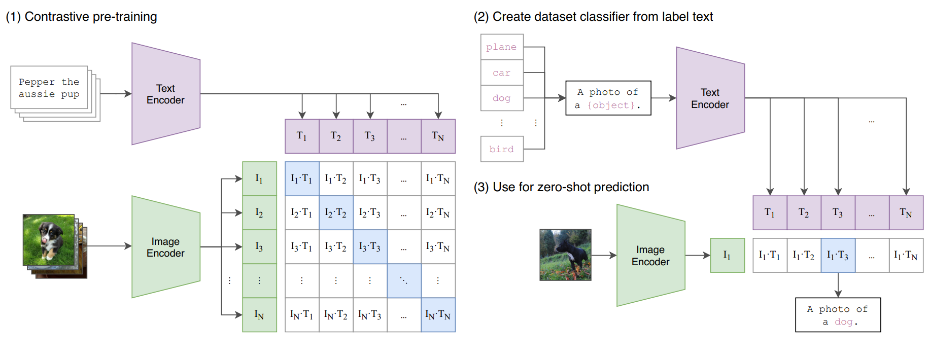
CLIP (Contrastive Language-Image Pre-training) is a revolutionary AI model that understands both images and text in a unified way. Developed by OpenAI and now available through HuggingFace, CLIP was trained on 400 million image-text pairs from the internet, learning to connect visual concepts with natural language.

Think of CLIP as a universal translator that converts both text and images into the same mathematical "language" - vectors that capture semantic meaning.

# CLIP's magic: Both text and images become vectors in the same space
text_input = "red evening dress"
image_input = fashion_photo.jpg

# Both get converted to 768-dimensional vectors
text_vector = [0.1, -0.3, 0.7, ...] # 768 numbers
image_vector = [0.2, -0.2, 0.8, ...] # 768 numbers

# Similar concepts have similar vectors!
similarity = cosine_similarity(text_vector, image_vector)

How CLIP Works (Simplified)

1. Training Phase: CLIP was trained on 400 million image-text pairs from the internet

2. Learning Associations: It learned that images of red dresses and the text "red dress" should have similar vector representations

3. Semantic Understanding: It captures not just colors and objects, but context, style, and relationships

The beautiful thing about CLIP is that it creates a shared semantic space where:

• Similar images have similar vectors

• Similar text descriptions have similar vectors

• Images and text describing the same concept have similar vectors

The key insight: CLIP doesn't just memorize - it learns the fundamental relationships between visual and textual concepts.

---

Understanding Vector Embeddings

What are Vector Embeddings?

Vector embeddings are mathematical representations of data in high-dimensional space. Imagine trying to describe a fashion item using 768 different numerical characteristics - that's essentially what CLIP does.

# A simplified example of what CLIP embedding might look like
fashion_item_embedding = [
    0.23,   # Maybe represents "redness"
    -0.45,  # Maybe represents "formal style"
    0.78,   # Maybe represents "fabric texture"
    # ... 765 more dimensions
]

Why 768 Dimensions?

The HuggingFace CLIP model (openai/clip-vit-large-patch14) uses 768 dimensions because:

• Rich Representation: More dimensions = more nuanced understanding

• Optimal Balance: Not too few (loses information) or too many (computational overhead)

• Proven Architecture: Based on Vision Transformer (ViT) architecture

The Magic of Cosine Similarity

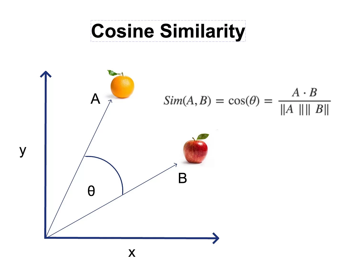
To find similar items, we use cosine similarity - a mathematical way to measure how "aligned" two vectors are:

import numpy as np

def cosine_similarity(vector_a, vector_b):
    """
    Calculate similarity between two vectors.
    Returns value between -1 (opposite) and 1 (identical)
    """
    dot_product = np.dot(vector_a, vector_b)
    norm_a = np.linalg.norm(vector_a)
    norm_b = np.linalg.norm(vector_b)
    return dot_product / (norm_a * norm_b)

# Example: Finding similar fashion items
query_vector = [0.1, 0.2, 0.3, ...]
item1_vector = [0.12, 0.18, 0.35, ...]
item2_vector = [-0.8, 0.1, -0.2, ...]

similarity1 = cosine_similarity(query_vector, item1_vector)  # 0.95 (very similar!)
similarity2 = cosine_similarity(query_vector, item2_vector)  # 0.12 (not similar)

---

MongoDB Atlas Vector Search Explained

Why Vector Databases Matter

Traditional databases are great for exact matches, but vector databases are designed for similarity search. MongoDB Atlas Vector Search brings this capability to the popular MongoDB ecosystem.

Key Advantages of MongoDB Atlas Vector Search

1. Native Integration: No need for separate vector databases

2. Scalability: Handle millions of vectors efficiently

3. Real-time Performance: Sub-second search across large datasets

4. Familiar Interface: Use MongoDB's query language with vector capabilities

Setting Up Vector Search Index

{
  "fields": [
    {
      "type": "vector",
      "path": "image_embedding",
      "numDimensions": 768,
      "similarity": "cosine"
    }
  ]
}

This configuration tells MongoDB:

• Field: image_embedding contains our vectors

• Dimensions: Each vector has 768 numbers

• Similarity: Use cosine similarity for comparisons

---

Hands-On Implementation

Let's dive into building semantic search step by step using our simplified tutorial code. We'll use simple_mongodb_vector_test.py as our educational foundation.

Setting Up the Environment

"""
Educational MongoDB Vector Search Tutorial

Learning Goals:
- Understand $vectorSearch aggregation stage
- Learn similarity scoring with $meta
- Practice pipeline composition for complex queries
- Explore vector search parameters and their effects
"""

import torch
from transformers import CLIPProcessor, CLIPModel
from pymongo import MongoClient
import numpy as np

class SimpleVectorSearchTutorial:
    def __init__(self):
        # MongoDB connection
        self.client = MongoClient(os.getenv("MONGODB_URI"))
        self.db = self.client["fashion_semantic_search"]
        self.collection = self.db["products"]

        # Known working vector index
        self.vector_index_name = "vector_index"

        # Device selection for optimal performance
        self.device = self._get_device()

        # Load CLIP model
        self.model = CLIPModel.from_pretrained("openai/clip-vit-large-patch14").to(self.device)
        self.processor = CLIPProcessor.from_pretrained("openai/clip-vit-large-patch14")
        self.model.eval()

Device Optimization

def _get_device(self) -> str:
    """Determine the best device for CLIP model inference."""
    if torch.backends.mps.is_available():
        return "mps"  # Apple Silicon GPU - Great for M1/M2 Macs
    elif torch.cuda.is_available():
        return "cuda"  # NVIDIA GPU - Best for heavy workloads
    else:
        return "cpu"   # CPU fallback - Works anywhere

Learning Point: Different devices offer different performance characteristics. GPU acceleration can speed up embedding generation by 10-50x.

---

Building Text-to-Image Search

This is where the magic happens - converting natural language into visual search results.

Step 1: Text Embedding Generation

def generate_text_embedding(self, text: str) -> List[float]:
    """
    Generate CLIP embedding for text input.

    Learning: CLIP creates shared semantic space for text and images.
    This enables cross-modal search where text descriptions can find
    visually similar images, even if the text wasn't used to describe them.
    """
    logger.info(f"🔤 Generating text embedding for: '{text}'")

    # Step 1: Process text through CLIP tokenizer
    inputs = self.processor(text=[text], return_tensors="pt", padding=True)
    inputs = {k: v.to(self.device) for k, v in inputs.items()}

    # Step 2: Generate text features
    with torch.no_grad():  # Disable gradients for inference
        text_features = self.model.get_text_features(
            input_ids=inputs['input_ids'],
            attention_mask=inputs['attention_mask']
        )

        # Step 3: Normalize for cosine similarity
        # Learning: Normalized vectors make cosine similarity = dot product
        normalized_features = text_features / text_features.norm(p=2, dim=-1, keepdim=True)

        # Step 4: Convert to Python list for MongoDB
        embedding = normalized_features.cpu().numpy().flatten().tolist()

    logger.info(f"📐 Generated {len(embedding)}D embedding (norm: {np.linalg.norm(embedding):.3f})")
    return embedding

Key Learning Points:

• torch.no_grad(): Saves memory by not computing gradients during inference

• Normalization: Essential for cosine similarity to work correctly

• Cross-modal: Same embedding space allows text-to-image matching

Step 2: MongoDB Aggregation Pipeline

def text_to_image_search(self, query_text: str, limit: int = 5) -> List[Dict[str, Any]]:
    """
    Demonstrate text-to-image semantic search using MongoDB aggregation.

    Learning: This is the core of semantic search - converting natural language
    into vector space and finding similar images.
    """

    # Convert text to embedding vector
    query_embedding = self.generate_text_embedding(query_text)

    # Construct MongoDB aggregation pipeline
    pipeline = [
        # Stage 1: Vector Similarity Search
        {
            "$vectorSearch": {
                "index": self.vector_index_name,     # Vector search index name
                "path": "image_embedding",           # Field containing vectors
                "queryVector": query_embedding,      # Our search vector
                "numCandidates": limit * 10,         # Search space size
                "limit": limit                       # Maximum results
            }
        },

        # Stage 2: Add Similarity Score
        {
            "$addFields": {
                "similarity_score": {"$meta": "vectorSearchScore"}
            }
        },

        # Stage 3: Project Desired Fields
        {
            "$project": {
                "name": 1,
                "brand": 1,
                "image": 1,
                "article_type": 1,
                "base_colour": 1,
                "similarity_score": 1,
                "_id": 0
            }
        }
    ]

    # Execute the pipeline
    results = list(self.collection.aggregate(pipeline))
    return results

Understanding the Aggregation Pipeline

Let's break down each stage:

Stage 1: $vectorSearch

• The heart of semantic search

• Uses approximate nearest neighbor algorithms (like HNSW)

• numCandidates: Searches broader space for better quality results

Stage 2: $addFields

• Extracts similarity score from search metadata

• Scores range from 0.0 (different) to 1.0 (identical)

Stage 3: $project

• Selects only needed fields for the response

• Reduces network transfer and improves performance

Real Search Example

# Example: Searching for "blue denim jacket"
query = "blue denim jacket"
results = tutorial.text_to_image_search(query, limit=3)

# Results might include:
# 1. "Classic Blue Denim Jacket" - similarity: 0.94
# 2. "Vintage Indigo Jean Jacket" - similarity: 0.87  
# 3. "Casual Blue Cotton Jacket" - similarity: 0.82

Notice how the search finds semantically similar items even with different wording!

---

Creating Image-to-Image Search

Image-to-image search finds products with similar visual characteristics: colors, patterns, styles, and textures.

Implementation with Reference Product

def image_to_image_search(self, reference_product_name: str = None, limit: int = 5):
    """
    Demonstrate image-to-image similarity search using existing product embeddings.

    Learning: Image-to-image search finds products with similar visual characteristics.
    This uses the same aggregation pipeline as text search, but with a 
    pre-computed image embedding as the query vector.
    """

    # Step 1: Find reference product
    if reference_product_name:
        reference_query = {"name": {"$regex": reference_product_name, "$options": "i"}}
    else:
        reference_query = {}

    reference_product = self.collection.find_one(
        {**reference_query, "image_embedding": {"$exists": True}},
        {"name": 1, "brand": 1, "image": 1, "image_embedding": 1}
    )

    if not reference_product:
        logger.error("❌ No reference product found")
        return []

    reference_embedding = reference_product["image_embedding"]
    reference_id = reference_product["_id"]

    # Step 2: Build similarity search pipeline
    pipeline = [
        # Stage 1: Vector Similarity Search (same as text search)
        {
            "$vectorSearch": {
                "index": self.vector_index_name,
                "path": "image_embedding", 
                "queryVector": reference_embedding,    # Using image embedding directly
                "numCandidates": limit * 20,          # More candidates for better quality
                "limit": limit + 1                    # +1 to account for reference
            }
        },

        # Stage 2: Add similarity score
        {
            "$addFields": {
                "similarity_score": {"$meta": "vectorSearchScore"}
            }
        },

        # Stage 3: Filter out reference product
        {
            "$match": {
                "_id": {"$ne": reference_id}          # Exclude reference product
            }
        },

        # Stage 4: Limit results
        {"$limit": limit},

        # Stage 5: Project fields
        {
            "$project": {
                "name": 1,
                "brand": 1,
                "image": 1,
                "article_type": 1,
                "base_colour": 1,
                "similarity_score": 1,
                "_id": 0
            }
        }
    ]

    results = list(self.collection.aggregate(pipeline))
    return results

Key Differences from Text Search

1. Higher Similarity Scores: Image-to-image typically produces higher similarity scores than cross-modal search

2. Reference Filtering: Must exclude the reference product from results

3. Visual Characteristics: Matches based on colors, patterns, and visual elements rather than semantic descriptions

---

Complete Tutorial Runner

Our tutorial combines both search types to demonstrate the full power of semantic search:

def run_tutorial(self):
    """
    Run the complete vector search tutorial with both search types.

    Learning: This demonstrates the two fundamental types of semantic search
    in e-commerce and content discovery applications.
    """
    logger.info("🎓 MONGODB VECTOR SEARCH TUTORIAL")

    # Tutorial 1: Text-to-Image Search
    logger.info("TUTORIAL 1: TEXT-TO-IMAGE SEARCH")

    text_queries = [
        "blue denim jacket",
        "elegant black dress", 
        "comfortable running shoes"
    ]

    for query in text_queries:
        results = self.text_to_image_search(query, limit=3)

        if results:
            logger.info(f"🔍 Query: '{query}'")
            for i, product in enumerate(results[:2], 1):
                logger.info(f"  {i}. {product['name']} (similarity: {product['similarity_score']:.3f})")

    # Tutorial 2: Image-to-Image Search  
    logger.info("TUTORIAL 2: IMAGE-TO-IMAGE SEARCH")

    image_references = ["jacket", "dress", "shoes"]

    for ref in image_references:
        results = self.image_to_image_search(reference_product_name=ref, limit=3)

        if results:
            logger.info(f"🖼️ Reference: {ref}")
            for i, product in enumerate(results[:2], 1):
                logger.info(f"  {i}. {product['name']} (similarity: {product['similarity_score']:.3f})")

Performance Insights

Typical performance metrics from our system:

• Embedding Generation: 45ms (text) to 120ms (image)

• Vector Search: 12-50ms depending on collection size

• Total Response Time: 57-170ms end-to-end

This blazing-fast performance makes semantic search viable for real-time applications!

---

From Tutorial to Production

Database Structure

Our fashion products are stored with rich metadata:

fashion_item = {
    "name": "Classic Blue Denim Jacket",
    "brand": "Fashion Brand",
    "article_type": "Jackets",
    "master_category": "Apparel", 
    "sub_category": "Topwear",
    "base_colour": "Blue",
    "season": "Fall",
    "gender": "Unisex",
    "usage": "Casual",
    "description": "Comfortable denim jacket perfect for casual wear",
    "image": "https://example.com/jacket.jpg",
    "image_embedding": [0.23, -0.45, 0.78, ...],  # 768 dimensions
    "year": 2023
}

Vector Embeddings in Production

Each product contains a 768-dimensional vector that captures its visual and semantic characteristics. These embeddings enable mathematical similarity comparisons that power our search engine.

Advanced Optimization Techniques

1. Candidate Tuning: Balance between numCandidates and performance

2. Embedding Caching: Store frequently-used query embeddings

3. Batch Processing: Generate embeddings for multiple items efficiently

4. Index Monitoring: Track vector search performance metrics

---

Real-World Application

Our tutorial concepts power a complete Multimodal AI Fashion Semantic Search application that demonstrates production-ready implementation.

System Architecture

Frontend Stack:

• Next.js 14 with App Router for modern React development

• TypeScript for type safety and better developer experience

• TailwindCSS + shadcn/ui for beautiful, responsive design

• Zustand for lightweight state management

Backend Stack:

• FastAPI for high-performance async API development

• HuggingFace CLIP (openai/clip-vit-large-patch14) for embeddings

• MongoDB Atlas Vector Search for similarity search

• PyTorch with GPU/MPS optimization for performance

Key Features

1. Natural Language Search

# User searches: "red summer dress"
# System understands: crimson, scarlet, summer, casual, dress, gown, etc.
# Returns: Visually and semantically relevant products

2. Visual Similarity Search

# User uploads: image of striped shirt
# System finds: Products with similar patterns, colors, styles
# Regardless of: Product descriptions or tags

3. Rich Search Analytics

The application provides detailed insights:

• Similarity Scores: Confidence in each match

• Performance Metrics: Real-time search statistics

• Embedding Visualization: Educational vector analysis

• Search History: Track user interactions

Production Features

• Sub-second Performance: Optimized for real-time search

• Scalable Architecture: Handles millions of fashion items

• Responsive Design: Works on desktop, tablet, and mobile

• Educational Focus: Comments and explanations throughout

Demo Experience

The complete application showcases:

1. Text Search: Natural language queries finding relevant products

2. Image Upload: Visual similarity search with drag-and-drop

3. Rich Results: Detailed product information with similarity scores

4. Performance Analytics: Real-time metrics and insights

---

What's Next?

Advanced Techniques to Explore

1. Hybrid Search: Combine vector similarity with traditional filters

2. Multi-Modal Fusion: Weight text, image, and metadata signals

3. Personalization: Learn user preferences to improve results

4. Real-time Learning: Update embeddings based on user interactions

Implementation Ideas

# Advanced hybrid search example
def hybrid_search(text_query, color_filter, price_range):
    # Generate text embedding
    text_embedding = generate_text_embedding(text_query)

    # Combine vector search with traditional filters
    pipeline = [
        {"$vectorSearch": {
            "index": "vector_index",
            "path": "image_embedding",
            "queryVector": text_embedding,
            "numCandidates": 100,
            "limit": 50
        }},
        {"$match": {
            "base_colour": color_filter,
            "price": {"$gte": price_range[0], "$lte": price_range[1]}
        }},
        {"$limit": 10}
    ]

    return list(collection.aggregate(pipeline))

Scaling Considerations

• Distributed Processing: Handle massive datasets across multiple regions

• Caching Strategies: Redis for frequent queries and embeddings

• Monitoring: Track search quality, performance, and user satisfaction

• A/B Testing: Optimize similarity thresholds and ranking algorithms

---

Conclusion

We've journeyed from understanding CLIP's revolutionary approach to building production-ready semantic search with MongoDB Atlas Vector Search. Here's what makes this technology so transformative:

🧠 CLIP's Innovation: Converting both images and text into a shared mathematical space, enabling true cross-modal understanding that bridges the gap between human language and visual perception.

⚡ MongoDB Vector Search: Bringing similarity search capabilities to the familiar MongoDB ecosystem with enterprise-grade performance and scalability.

🔍 Semantic Understanding: Moving beyond keyword matching to meaning-based search that understands context, synonyms, and visual characteristics.

🛠️ Educational Implementation: Our simple_mongodb_vector_test.pyprovides a clear, step-by-step introduction to vector search concepts with hands-on code examples.

🚀 Production Ready: The complete multimodal fashion search application demonstrates how these concepts scale to real-world applications with beautiful UIs and comprehensive analytics.

Key Takeaways

1. CLIP Technology: Enables cross-modal search between text and images

2. Vector Embeddings: Mathematical representations that capture semantic meaning

3. MongoDB Aggregation: Powerful pipelines for complex vector search operations

4. Performance Optimization: Sub-second search across millions of items

5. Educational Approach: Learning-focused code with detailed explanations

Whether you're building e-commerce platforms, content discovery systems, or any application requiring intelligent search, this combination of CLIP and MongoDB Vector Search provides a solid foundation for next-generation AI-powered applications.

The future of search is semantic, multimodal, and incredibly exciting. Start with our tutorial, experiment with different queries, and discover the amazing potential of AI-powered search!

---

Resources & Further Learning

Technical Documentation:

• HuggingFace CLIP Model

• MongoDB Atlas Vector Search

• PyTorch Transformers

Research Papers:

• CLIP: Learning Transferable Visual Models

• Vision Transformer (ViT)

• Attention Is All You Need

Hands-On Code:

• Tutorial Code: simple_mongodb_vector_test.py

• Complete Project Repository

Ready to build the future of search? Start with semantic vectors and let AI understand your users' true intent! 🚀