Hey everyone! 👋

I am a student who just started his journey in Machine Learning and Artificial Intelligence few months ago. And I was recently learning about Artificial Neural Network(ANN), and while exploring various tutorials and articles, I realized that although the basics were covered in them but I still lacked a deeper understanding of how ANNs actually work. So that’s when I decided to take a challenge: to build a neural network from scratch using only Python and NumPy. No TensorFlow, no PyTorch — just pure mathematics and code to really grasp what’s happening under the hood.

Why?

While frameworks like TensorFlow ,Keras and PyTorch make it easy to create neural networks, I realized that building one from scratch was essential to truly understanding how they work.

One day, while browsing through Youtube, I stumbled upon a video tutorial explaining how to implement a simple neural network from scratch. It was a bit intimidating at first, as there was a lot of math and code to digest — but it also sparked an idea in me. What if I also try to build my own neural network line by line from complete scratch? By doing so, I would truly understand how forward propagation, backpropagation, and all other elements fit together to form a working model.

🎯 Personal Goal*: Understand every single line of code I write, not just copy-paste from tutorials!*

In this blog post, I’ll share my journey of implementing a neural network for digit recognition using only NumPy, and try my best to break down both the mathematics and the code, and explaining how each component fits together.

My starting Point

Before diving in, here’s what I knew:

• Basic python programming.

• Familiar with NumPy, but not at an advanced level.

• Basic Mathematics: Calculus and Linear Algebra.

• A basic understanding of how neural network works.

Choosing a dataset

Once I decided to build my own neural network, the next step was to choose a dataset. Digit recognition is a common example used in many tutorials and articles, and it seemed like a logical place to start. After some research, I settled on the MNIST dataset, which is widely used for this very purpose.

Interestingly, I had already worked with the MNIST dataset while reading the book “Hands-On Machine Learning with Scikit-Learn, Keras, and TensorFlow”, so it felt like a familiar starting point for my project.

💡 Fun Fact*: The MNIST dataset is often considered the **“Hello World”** of machine learning. It’s used by data scientists to train algorithms as a simple way to test new architectures or frameworks and ensure they work properly.*

Understanding the Dataset

Before starting to code and build the neural network, it’s essential to spend a fair amount of time understanding the dataset on which we will work. This knowledge will help make the model more effective.

Here’s what I learned about the MNIST dataset:

• Dataset Overview: The dataset contains 70,000 handwritten digit images, each sized at 28x28 pixels. Each image is paired with a label that indicates the digit it represents (from 0 to 9), which is crucial for supervised learning.

• Train/Test Split: The dataset is typically divided into a training set (60,000 images) and a test set (10,000 images). This split allows us to evaluate the performance of the model after training.

• Data Format: Each image is represented as a 28x28 array of grayscale pixel values, ranging from 0 (black) to 255 (white).

Setting up My Environment

Since my old laptop has a habit of heating up and running slowly, I decided to take my coding to Kaggle. It’s a fantastic platform that gives me access to powerful hardware for training my models and lets me save my dataset and code in the cloud. This way, I can easily access my projects from anywhere without worrying about my laptop overheating. Plus, the community and built-in notebooks are super helpful for getting tips and improving my models!

So, Let’s Start —

Required Libraries:

For this project, I needed only two key and one extra library:

1. NumPy: For numerical operations and array handling.

2. Pandas: For importing the MNIST data from a CSV file.

3. Matplotlib: For displaying the images of handwritten digits.

Code-

import numpy as np
import pandas as pd
import matplotlib.pyplot as plt

I imported the libraries NumPy, Pandas, and Matplotlib as np, pd, and plt respectively. This makes our code cleaner and easier to work with as we move forward. Plus, using shorter names is a common practice that enhances readability!

Loading the Dataset

The MNIST dataset is readily available in several formats, but for this blog, I used the CSV version. Here’s how I loaded the dataset:

# Load the dataset
data = pd.read_csv('path_to_mnist_training_data.csv')

After loading the data, I converted pandas DataFrame into a NumPy array for easier manipulation. The dataset is organized such that the first column represents the labels (the digit each image represents), and the remaining columns represent the pixel values of the images.

# Converting the DataFrame to a NumPy array for easier manipulation
data = np.array(data)

Preparing the data

Before diving into the neural network implementation, I needed to preprocess the data. This involves various steps:

• Getting the shape of the data- number of samples(m) and features(n):

m, n = data.shape

• Shuffling the data to ensure randomness in training:

np.random.shuffle(data)

• Separating the data into validation data and training data and their labels and features and normalizing input data.

data_dev = data[0:1000].T         # Development set of 1000 samples
Y_dev = data_dev[0]               # Labels for the development set
X_dev = data_dev[1:n]             # Features for the development set
X_dev = X_dev / 255               # Normalizing the input data

data_train = data[1000:m].T       # Training set
Y_train = data_train[0]           # Labels for the training set
X_train = data_train[1:n]         # Features for the training set
X_train = X_train / 255           # Normalizing the input data

I divided the data into the validation set because it is important for Hyperparameter tuning and prevent overfitting.(At first I totally forgot this step)

Normalizing the pixel values (scaling them between 0 and 1) helps the model converge faster during training.

Deciding the Neural Network(NN) Architecture

Before jumping into the coding Neural Network, I had to plan out the architecture of the Neural Network I was going to build. Initially, I started with a simple setup consisting of an input layer, one hidden layer with 10 neurons, and an output layer with 10 neurons (one for each digit class, representing digits 0–9). However, I realized that by tweaking the architecture, I could improve the accuracy of my model.

After some experimentation, I opted for a slightly more complex architecture, which improved the model’s accuracy by roughlt 4–5%. Here’s the structure I ended up with:

Neural Network Architecture

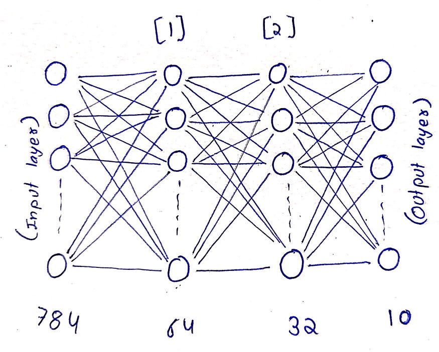
Neural Network Structure

1. Input Layer:

• Size: 784 neurons (since each MNIST image is 28x28 pixels, and 28 × 28 = 784).

• Purpose: This layer holds the pixel values of the input image, flattened into a vector.

2. First Hidden Layer

• Size: 64 neurons.

• Activation Function: ReLU (Rectified Linear Unit).

• Weights: W1 (randomly initialized matrix of size 64x784).

• Biases: b1 (randomly initialized vector of size 64x1).

• Forward Propagation:

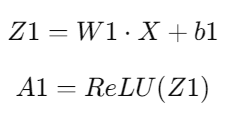
Where:

• Z1 — weighted sum of the inputs.

• W1​ — weight matrix for the first layer (with size 64x784).

• X — input vector (with size 784x1).

• b1​ — bias vector (with size 64x1).

3. Second Hidden Layer

• Size: 32 neurons.

• Activation Function: ReLU.

• Weights: W2 (randomly initialized matrix of size 32x64).

• Biases: b2 (randomly initialized vector of size 32x1).

• Forward Propagation:

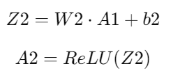
Where:

• Z2 — weighted sum of the output from the first hidden layer.

• W2 — weight matrix for the second layer (size 32x64).

• A1 — output from the first hidden layer (size 64x1).

• b2 — bias vector (size 32x1).

4. Output Layer

• Size: 10 neurons (one for each class, as MNIST has 10 digit classes: 0–9).

• Activation Function: Softmax.

• Weights: W3 (randomly initialized matrix of size 10x32).

• Biases: b3 (randomly initialized vector of size 10x1).

• Forward Propagation:

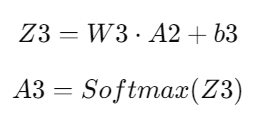
Where:

• Z3 — weighted sum of the outputs from the second hidden layer.

• W3 — weight matrix for the output layer (size 10x32).

• A2 — output from the second hidden layer (size 32x1).

• b3 — bias vector (size 10x1).

Summary of the Architecture

• Input Layer: 784 neurons (input pixel values).

• Hidden Layer 1: 64 neurons, ReLU activation.

• Hidden Layer 2: 32 neurons, ReLU activation.

• Output Layer: 10 neurons, Softmax activation (for classification into 10 classes).

Input (784) → Hidden1 (64) → Hidden2 (32) → Output (10)
     ↓              ↓              ↓              ↓
   Raw       →    ReLU      →    ReLU     →   Softmax
  Pixels       Activation    Activation    Activation

Why ReLU and Softmax and what do they do?

ReLU (Rectified Linear Unit)

It is used in hidden layers because it introduces non-linearity, helping the network learn complex patterns. It’s computationally efficient and avoids the vanishing gradient problem, allowing the network to learn faster.

It is an activation function that returns the input directly if it’s positive; otherwise, it returns zero. Mathematically:

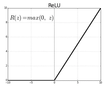
This means:

• if Z > 0, ReLU(Z) = Z

• if Z < 0, ReLU(Z) = 0

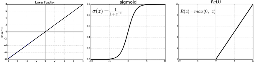
In this case, I chose not to use a linear function because it would behave similarly to linear regression, limiting the network’s ability to detect complex patterns. I also avoided the sigmoid function, as it can complicate the model and isn’t the best choice for simple use cases due to issues like vanishing gradients. Instead, I opted for the ReLU function, which is not only easier to implement but also speeds up the network’s training process. Additionally, ReLU introduces non-linearity into the model, allowing it to learn more complex relationships in the data.

Softmax

Softmax is used in the output layer for classification tasks, converting the raw output (logits) into probabilities. It ensures that the probabilities of all classes sum to 1, making it easy to interpret the network’s prediction by selecting the class with the highest probability.

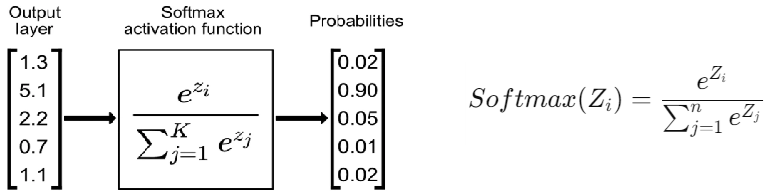
Where:

• Zi — raw score (logit) for class i,

• n — total number of classes (in our case, n=10, since MNIST has 10 digit classes).

In short, ReLU helps the network learn, and Softmax makes its predictions interpretable.

Initializing parameters

Next, I needed to initialize the weights and biases for my neural network. This step is crucial, as the initial values can affect how well the model learns and during training model the values change and for changing we need to have some initial values.

def initialize_parameters():
    """Initializes the parameters (weights and biases) for the neural network."""
    W1 = np.random.rand(64, 784) - 0.5   # Weights for the first layer (64 neurons, 784 inputs)
    b1 = np.random.rand(64, 1) - 0.5     # Bias for the first layer
    W2 = np.random.rand(32, 64) - 0.5    # Weights for the second layer (32 neurons, 64 inputs)
    b2 = np.random.rand(32, 1) - 0.5     # Bias for the second layer
    W3 = np.random.rand(10, 32) - 0.5    # Weights for the output layer (10 neurons, 32 inputs)
    b3 = np.random.rand(10, 1) - 0.5     # Bias for the output layer
    return W1, b1, W2, b2, W3, b3

Here, I initialized the weights randomly between -0.5 to 0.5.

It took me some time to fully grasp the shapes of the matrices and how they interact and operate with one another. At first, the shapes were really confusing, but after experimenting with them multiple times, I finally figured it out.

Start Training process of the Neural Network

Now, with the architecture set up, it was time to implement the training loop using forward propagation, backpropagation, and gradient descent. These steps are crucial for optimizing the network’s parameters (weights and biases) so that it can minimize the error in its predictions.

Forward Propagation

Now let’s start with the forward propagation step. In this process input data moves through the network layers, and model make predictions based on the learned parameters.

At each layer, a linear transformation is applied to the inputs, followed by an activation function to introduce non-linearity. Here’s how I implemented it and activation functions:

def ReLU(Z):
    return np.maximum(Z, 0)

def softmax(Z):
    A = np.exp(Z) / sum(np.exp(Z))
    return A

def forward_prop(W1, b1, W2, b2, W3, b3, X):
    Z1 = W1.dot(X) + b1     # Linear transformation for the first layer
    A1 = ReLU(Z1)           # Activation function for the first layer
    Z2 = W2.dot(A1) + b2    # Linear transformation for the second layer
    A2 = ReLU(Z2)           # Activation function for the second layer
    Z3 = W3.dot(A2) + b3    # Linear transformation for the output layer
    A3 = softmax(Z3)        # Applying softmax to get output probabilities
    return Z1, A1, Z2, A2, Z3, A3

The input passes through each layer, and I apply the ReLU activation function in the hidden layers and softmax at the output. This ensures that each layer transforms the input data appropriately before passing it to the next layer.

Now, I coded the 2 more essential functions — ReLU derivative and the one hot encoder. These 2 functions are used in backward propagation.

def ReLU_deriv(Z):
  return Z > 0

def one_hot(Y):
    one_hot_Y = np.zeros((Y.size, Y.max() + 1))
    one_hot_Y[np.arange(Y.size), Y] = 1
    one_hot_Y = one_hot_Y.T
    return one_hot_Y

ReLU_deriv is a function to calculate the derivative of ReLU function.

one_hotis function for One Hot Encoding. It converts each label into binary vector where correct class is marked as 1 and other as 0. For example, the label “2” becomes [0, 0, 1, 0, 0, 0, 0, 0, 0, 0].

Backward Propagation

Now after building the structure for the network it’s time to teach the network to recognize the digits from the 28x28 pixel image. Backpropagation is the process that allows the network to learn by adjusting its parameters based on the error in its predictions. Backpropagation moves in reverse from direction of output layer to input layer.

The basic outline:

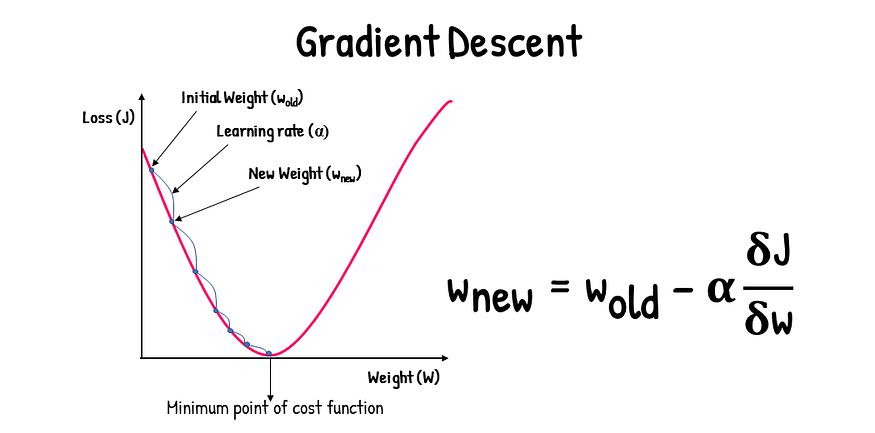
1. Compute the Loss: First, we calculate the loss, which is the difference between the predicted and actual values. This gives us a measure of how wrong the network’s predictions are.

2. Adjust the Parameters: We then minimize this loss by adjusting the network’s weights and biases. This is done using a technique called gradient descent, where we update the parameters in the direction that reduces the error the most.

3. Repeat the Process: This process of computing the loss and adjusting the parameters is repeated multiple times. Over time, the network gradually improves its accuracy and becomes better at recognizing the digits.

Now, let’s break down the code for backward propagation:

def backward_prop(Z1, A1, Z2, A2, Z3, A3, W1, W2, W3, X, Y):
    one_hot_Y = one_hot(Y)      # Convert labels to one-hot encoding
    dZ3 = A3 - one_hot_Y        # Compute the gradient for the output layer
    dW3 = 1 / m * dZ3.dot(A2.T) # Gradient for weights of output layer
    db3 = 1 / m * np.sum(dZ3)   # Gradient for biases of output layer

    # Backpropagate through the second layer
    dZ2 = W3.T.dot(dZ3) * ReLU_deriv(Z2)
    dW2 = 1 / m * dZ2.dot(A1.T)   # Gradient for weights of second layer
    db2 = 1 / m * np.sum(dZ2)     # Gradient for biases of second layer

    # Backpropagate through the first layer
    dZ1 = W2.T.dot(dZ2) * ReLU_deriv(Z1)
    dW1 = 1 / m * dZ1.dot(X.T)     # Gradient for weights of first layer
    db1 = 1 / m * np.sum(dZ1)      # Gradient for biases of first layer

    return dW1, db1, dW2, db2, dW3, db3

Explanation:

The backward_prop function computes and returns the gradients for each layer in the network.

• dZ3, dW3, db3: These represent the gradients for the output layer, calculated using the difference between the network’s prediction (A3) and the true labels (converted to one-hot format).

• dZ2, dW2, db2: These are the gradients for the second layer, calculated by backpropagating the error from the output layer through the weights of the second layer.

• dZ1, dW1, db1: Similarly, these are the gradients for the first layer, backpropagating further from the second layer through the weights of the first layer.

Next, we update the parameters using the computed gradients:

def update_params(W1, b1, W2, b2, W3, b3, dW1, db1, dW2, db2, dW3, db3, alpha):
    """Updates the parameters using gradient descent."""
    W1 = W1 - alpha * dW1  # Update weights of the first layer
    b1 = b1 - alpha * db1   # Update biases of the first layer
    W2 = W2 - alpha * dW2   # Update weights of the second layer
    b2 = b2 - alpha * db2   # Update biases of the second layer
    W3 = W3 - alpha * dW3   # Update weights of the output layer
    b3 = b3 - alpha * db3   # Update biases of the output layer
    return W1, b1, W2, b2, W3, b3

Explanation:

The update_params function updates the network's weights and biases using the gradients calculated from backpropagation.

• W1, W2, W3: These represent the weights for the first, second, and output layers, respectively.

• b1, b2, b3: These represent the biases for the respective layers.

• alpha: This is the learning rate, which controls how much the parameters are adjusted during each update. A higher learning rate leads to faster updates but might overshoot the optimal values, while a smaller rate slows down the process but ensures more precise learning.

By adjusting the weights and biases in this way, the network reduces the loss and improves its accuracy over time.

Training the Neural Network Using Gradient Descent

Now as we have coded both the forward and backward propagation, next step is to train the network using gradient descent. Here’s what happens during the process:

1. Initialize Parameters: We start by initializing the weights and biases.

2. Forward and Backward Propagation: For each iteration, we compute the outputs through forward propagation and calculate the loss. Then, we perform backward propagation to adjust the weights and biases based on the error.

3. Update the Parameters: Using the gradients calculated from backpropagation, we update the parameters to minimize the loss.

4. Check Accuracy: We periodically check the accuracy of the network to see how well it’s learning.

Here’s the complete code for training the network:

def get_predictions(A3):
    return np.argmax(A3, 0)


def get_accuracy(predictions, Y):
    print(predictions, Y)    # Optional: Print predictions and true labels for inspection
    return np.sum(predictions == Y) / Y.size


def gradient_descent(X, Y, alpha, iterations):
    W1, b1, W2, b2, W3, b3 = initialize_parameters()
    for i in range(1, iterations+1):
        # Forward propagation
        Z1, A1, Z2, A2, Z3, A3 = forward_prop(W1, b1, W2, b2, W3, b3, X)

        # Backward propagation
        dW1, db1, dW2, db2, dW3, db3 = backward_prop(Z1, A1, Z2, A2, Z3, A3, W1, W2, W3, X, Y)

        # Update parameters
        W1, b1, W2, b2, W3, b3 = update_params(W1, b1, W2, b2, W3, b3, dW1, db1, dW2, db2, dW3, db3, alpha)

        # Print the progress every 50 iterations
        if i % 50 == 0:
            print("Iteration: ", i)
            predictions = get_predictions(A3)
            print("Accuracy: ", get_accuracy(predictions, Y))

    return W1, b1, W2, b2, W3, b3

Explanation:

• get_predictions: This function returns the class with the highest predicted probability for each sample.

• get_accuracy: It compares the predicted classes with the actual labels and calculates the accuracy of the network.

• gradient_descent: This is the main training loop where we perform forward and backward propagation and update the weights and biases using gradient descent. We also track the accuracy every 50 iterations to monitor the network’s progress.

By training the network using gradient descent, we gradually minimize the loss and improve the accuracy of the model. The final trained network should be able to recognize handwritten digits with a high degree of accuracy.

In the following code, we’ll train the network on the training set with a learning rate of 0.2 and for 500 iterations. The learning rate controls how large a step we take during each iteration towards minimizing the loss, and the number of iterations defines how many times the network will adjust its weights and biases to improve accuracy.

# Training the neural network on the training set
W1, b1, W2, b2, W3, b3 = gradient_descent(X_train, Y_train, 0.2, 500)

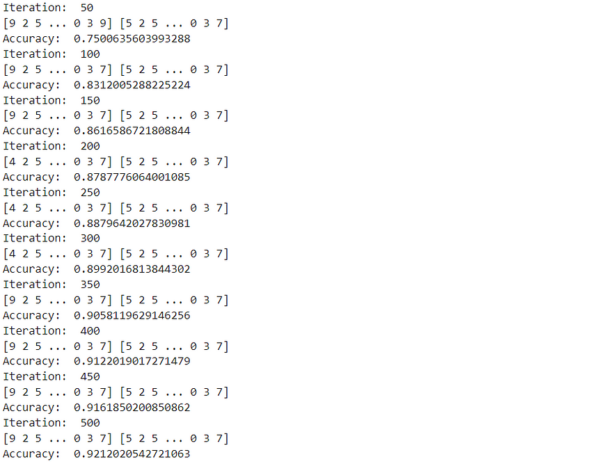
By running the above code, the neural network will start training on the training data (X_train and Y_train). As it trains, you’ll see the accuracy improving after every 50 iterations, as we’ve set it to print the progress during training. Once the training is complete, the network is ready to classify new images of handwritten digits with a good level of accuracy of about 92%.

It took about 3–5 minutes to train the network on the training data on kaggle.

The backpropagation and gradient descent concepts were quite challenging for me to digest and took the most time to fully understand out of the entire project. However, thanks to the Andrew Ng Machine Learning specialization course, I was able to grasp them more quickly than I would have otherwise. Without the course, I think it would have taken me days to fully comprehend these topics.

Making Predictions with the Trained Model

After training the neural network, the next step is to test the model’s ability to make predictions. For this, we will write two functions: one for generating predictions for the input data and another to visualize the predictions on specific images from the dataset.

The make_predictions function will use the trained weights and biases to compute the predictions for the input data.

def make_predictions(X, W1, b1, W2, b2, W3, b3):
  """Generates predictions for the input data using the trained network."""
  _, _, _, _, _, A3 = forward_prop(W1, b1, W2, b2, W3, b3, X)
  predictions = get_predictions(A3)
  return predictions

Next, the test_prediction function will allow us to test the model's prediction for a specific image from the training set, visualize the image, and compare the prediction with the actual label. This will help us see how well the model has learned to recognize digits.

def test_prediction(index, W1, b1, W2, b2, W3, b3):
      current_image = X_train[:, index, None]  # Get the current image (column vector)
      prediction = make_predictions(X_train[:, index, None], W1, b1, W2, b2, W3, b3)  # Get prediction for the current image
      label = Y_train[index]  # Get the true label for the current image
      print("Prediction: ", prediction)  # Print the predicted class
      print("Label: ", label)  # Print the true label

      # Reshape the image for displaying and scale back to 0-255
      current_image = current_image.reshape((28, 28)) * 255
      plt.gray()  # Set the colormap to gray
      plt.imshow(current_image, interpolation='nearest')  # Display the image
      plt.show()  # Show the plot

I tested this function by providing some indexes of an image from the training set, and the network will attempt to predict which digit it is, display the corresponding image, and its correct label.

indexes = [1,50,100,150,200,250,300,350,400,450]
for i in indexes:
  test_prediction(i, W1, b1, W2, b2, W3, b3)

Out of these 10 digits it almost predicted 9 correct and 1 incorrect.

Validation Set

In the journey of building machine learning models, understanding how to evaluate their performance is crucial. One of the key components of this evaluation is the validation set.

A validation set is a subset of your dataset used to tune your model’s hyperparameters. It’s distinct from the training set (for training the model) and the test set (for final evaluation). The main purpose of the validation set is to measure how well the model can generalize to unseen data.

Why Use a Validation Set?
During training, models can easily overfit, meaning they learn noise and outliers from the training data, which harms performance on new data. The validation set helps monitor the model’s performance during training and allows for adjustments to prevent overfitting.

So let’s check the model on the validation set:

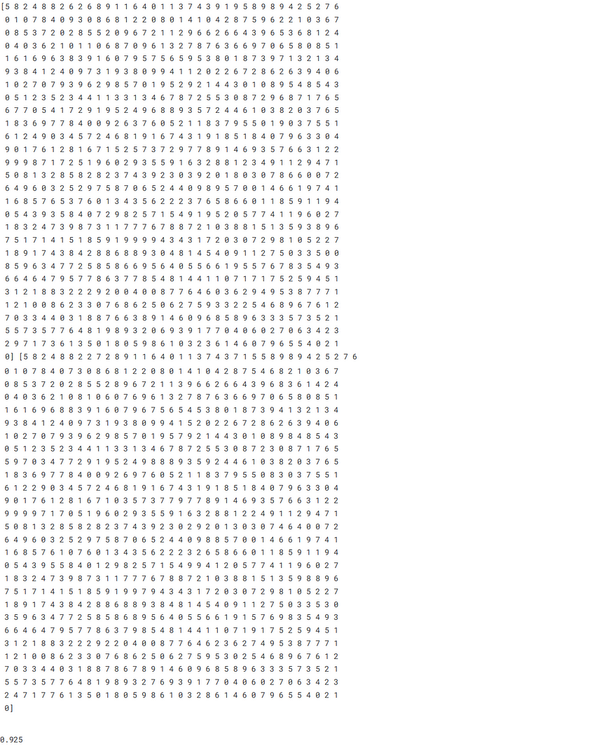
dev_predictions = make_predictions(X_dev, W1, b1, W2, b2, W3, b3)
get_accuracy(dev_predictions, Y_dev)

This step is crucial for improving the performance of the network as doing so helped me increase the network’s accuracy by 4–5%

Testing the Neural Network on Unseen Data

After training and validating our neural network, it’s time to see how well it performs on a separate set of unseen data — the test set. This helps evaluate how well the model generalizes to data it hasn’t seen during training. We’ll load the test dataset, prepare the data, and compute the model’s accuracy on this set.

First, let’s import the test data:

# Importing test data
test_data = pd.read_csv('path_to_test_data.csv')

Here, the test dataset is loaded from a CSV file and converted into a NumPy array for easier manipulation.

# Converting the test data to a NumPy array
test_data = np.array(test_data)

# Getting the number of samples (m_test) and features (n_test) from the test dataset
m_test, n_test = test_data.shape

Next, we will prepare the test data by separating the labels and features, then normalizing the features (just like we did with the training data):

# Preparing the test data
test_data_dev = test_data.T  # Transposing the test data for easier indexing
Y_test = test_data_dev[0]    # Labels for the test set
X_test = test_data_dev[1:n_test]  # Features for the test set
X_test = X_test / 255         # Normalizing the test input data (values between 0 and 1)

Now that the test data is ready, we can use the trained network to make predictions and calculate the accuracy:

# Making predictions on the test set and calculating accuracy
test_data_predictions = make_predictions(X_test, W1, b1, W2, b2, W3, b3)  # Get predictions for the test set
test_accuracy = get_accuracy(test_data_predictions, Y_test)  # Calculate accuracy for the test set
print("Test Set Accuracy: ", test_accuracy)  # Print the accuracy

This part of the code will predict the digits from the test dataset and compute the accuracy by comparing the predictions to the actual labels. The test accuracy will give us an indication of how well the model generalizes to new, unseen data.

After testing the network on the test data, I achieved approximately 92% accuracy, compared to about 84% with the previous architecture and . I believe accuracy can be further improved by fine-tuning the hyperparameters and experimenting with different architectural choices.

Conclusion

Building a neural network from scratch has been an exhilarating journey that deepened my understanding of machine learning while igniting my creativity. Throughout this process, I discovered the vital role each layer and parameter plays in making accurate predictions

I had often heard that writing a blog can enhance learning, but I didn’t truly believe it until I embarked on this writing adventure. Here are a few insights I gained along the way:

1. A deeper understanding of neural networks.

2. A bit of insight into the art of blog writing.

3. Improved English skills, particularly in expressing complex concepts clearly.

4. A clearer grasp of the mathematics and matrix manipulations involved.

Code:

If you want the code you can check my —

Kaggle notebook — https://www.kaggle.com/code/pankajgoyal4152/neural-network-from-scratch

GitHub Repo — https://github.com/Pankaj4152/Neural-Network

Next steps?

This project has been a great starting point, but I know there’s still a lot to learn. My next steps include:

• Deepening My Understanding: I plan to further my knowledge of neural networks and machine learning by studying more advanced concepts and techniques.

• Experimenting with Neural Network Architectures: I will explore various architectures by adding more hidden layers, experimenting with different activation functions, and adjusting hyperparameters. I’ll closely monitor how these changes impact performance and accuracy.

• Exploring Advanced Implementation Techniques: I’m excited to try a more advanced approach to implementing neural networks from scratch. This will give me a deeper insight into their mechanics and improve my overall skill set.

Final Thoughts 💭

Creating this neural network was challenging yet incredibly rewarding. It transformed abstract mathematical equations into tangible concepts I can now understand and apply. If you’re delving into machine learning, I highly recommend trying this yourself!

As this was my first blog, I may have made a few mistakes, and I appreciate your understanding as I strive to improve in future posts.

Confession time: I started this journey unsure of how to structure my writing, so I turned to ChatGPT and Claude for a basic layout. I then shaped the content and polished it further with some helpful guidance.

I’d love to hear your thoughts or questions in the comments below. If you’re also exploring machine learning or neural networks, let’s connect and share knowledge and experiences. Happy coding!

Let’s Connect:

• LinkedIn — https://www.linkedin.com/in/pankaj4152/

• GitHub —https://github.com/Pankaj4152