From Pixels to Patterns: A Deep Dive into Convolutional Neural Networks (CNNs)
 Tanayendu Bari
Introduction
Convolutional Neural Networks (CNNs) have dramatically transformed the landscape of computer vision, enabling machines to perceive and interpret visual data with unprecedented accuracy and efficiency. Initially developed for tasks like handwritten digit recognition, CNNs have since become the backbone of countless modern applications ranging from facial recognition, autonomous driving, and real-time object detection to medical imaging and industrial quality inspection. Their ability to automatically learn hierarchical spatial features directly from raw pixel data has set them apart from traditional hand-engineered feature-based approaches.
This blog aims to offer a deep yet accessible exploration of CNNs. We begin with the fundamental principles that govern their design and operation, followed by a historical overview of significant milestones and architectural breakthroughs. From the simplicity of LeNet to the sophistication of ConvNeXt, we will analyze how CNN architectures have evolved to become more powerful, efficient, and scalable. Whether you're a beginner curious about the building blocks or a practitioner seeking clarity on advanced trends, this guide serves as a comprehensive resource on CNNs in deep learning.
What Is Convolution?
Convolution is a fundamental operation in CNNs that combines local regions of the input image with a kernel (also called a filter) to produce feature maps. Unlike traditional matrix multiplication, convolution involves sliding the kernel across the input and computing a weighted sum at each location.
Mathematically, convolution involves flipping the kernel both horizontally and vertically and then performing element-wise multiplication and summation with the overlapping region of the image. If the kernel is symmetric, flipping is not necessary.
Example:
Given a 3x3 image patch and a 3x3 kernel:
$$\textbf{Image Patch:} \quad \begin{bmatrix} a & b & c \\ d & e & f \\ g & h & i \end{bmatrix} \qquad \textbf{Kernel:} \quad \begin{bmatrix} 1 & 2 & 3 \\ 4 & 5 & 6 \\ 7 & 8 & 9 \end{bmatrix}$$
The convolution result at the centre pixel is:
$$(i \cdot 1) + (h \cdot 2) + (g \cdot 3) + (f \cdot 4) + (e \cdot 5) + (d \cdot 6) + (c \cdot 7) + (b \cdot 8) + (a \cdot 9)$$
Pseudocode:
for each row in image:
    for each pixel in row:
        accumulator = 0
        for each kernel row:
            for each kernel col:
                accumulator += image value * corresponding kernel value
        set output pixel = accumulator
This process is repeated for each position of the kernel across the image. The centre of the kernel is aligned with the pixel being updated, and the resulting value is stored in the output feature map.
Convolution captures local spatial features like edges, corners, and textures, making it ideal for vision tasks.
Understanding Image Data
Digital images are essentially structured collections of pixels arranged in a two-dimensional grid. Each pixel represents the smallest unit of visual information and contains values that describe colour intensity. In most standard formats, these values are divided across three colour channels—Red, Green, and Blue (RGB). For grayscale images, a single channel is sufficient, whereas coloured images typically use three channels.
An image of size 256x256 pixels with three channels (RGB) is represented as a 3D matrix or tensor of shape (256, 256, 3). Each pixel in this grid holds an integer (or float) value ranging from 0 to 255 (in 8-bit format), indicating the brightness or intensity of that particular colour component.
Understanding how images are structured is crucial because CNNs operate directly on this 3D tensor format. The spatial relationships between pixels—such as edges, textures, and patterns—are preserved in the grid, allowing convolutional filters to detect low-level features (e.g., edges and corners) in early layers and complex features (e.g., shapes and objects) in deeper layers.
Additionally, real-world images often come in varying sizes and aspect ratios, so preprocessing steps such as resizing, normalization, and data augmentation are usually applied before feeding them into a CNN model.
Classical Vision vs CNNs
Before the rise of Convolutional Neural Networks (CNNs), computer vision systems relied heavily on manually designed feature extraction techniques to interpret image data. These classical methods used mathematical filters and algorithms to detect edges, textures, and shapes based on pixel intensity changes.
Edge Detection Filters
Sobel Filter :
The Sobel operator, also known as the Sobel–Feldman operator, is one of the earliest and most well-known edge detection methods in image processing. Proposed in 1968 by Irwin Sobel and Gary Feldman, it is a discrete differentiation operator that computes an approximation of the gradient of the image intensity function.
It uses two 3×3 kernels—one for horizontal changes and one for vertical changes:
Horizontal (Gx):
$$G_x = \begin{bmatrix} -1 & 0 & +1 \\ -2 & 0 & +2 \\ -1 & 0 & +1 \end{bmatrix} * A$$
Vertical (Gy):
$$G_y = \begin{bmatrix} -1 & -2 & -1 \\ 0 & 0 & 0 \\ +1 & +2 & +1 \end{bmatrix} * A$$
Here, * denotes 2D convolution with the image A. The result is an image that highlights intensity changes (edges) in the respective directions. These approximations can be combined to compute the gradient magnitude:
$$G = \sqrt{G_x^2 + G_y^2}$$
And the direction of the gradient can be computed as:
$$\quad \Theta = \operatorname{atan2}(G_y, G_x)$$
This method approximates gradients with built-in smoothing due to its filter design and is computationally efficient, but it’s relatively crude and sensitive to noise.
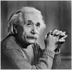
Here's a sample image to which we will apply both masks individually
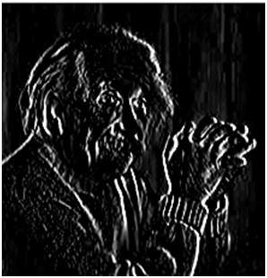
After Applying the vertical Mask:
After applying the Horizontal Mask:
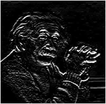
In the first image, where the vertical mask is applied, the vertical edges become more prominent compared to the original image. Similarly, in the second image, the horizontal mask highlights the horizontal edges effectively.
This demonstrates how both horizontal and vertical edges can be detected using appropriate edge detection masks. When comparing the results of the Sobel and Prewitt operators, you’ll notice that the Sobel operator typically produces more pronounced edges.
This is because the Sobel operator assigns greater weight to pixel intensities near the centre of the mask, enhancing the contrast along edges more effectively than the Prewitt operator.
Prewitt Filter:
The Prewitt filter is another early edge detection operator similar to the Sobel filter but with simpler coefficients. It also estimates the gradient of the image intensity at each point, indicating both the magnitude and direction of the sharpest change in brightness, which is typically used to detect edges.
In simple terms, it measures how abruptly or smoothly an image changes at each point, helping determine where an edge exists and how it's oriented. The gradient is represented by a 2D vector at each image point—pointing in the direction of the largest increase in brightness—and the vector’s magnitude indicates how steep the change is.
Like the Sobel operator, the Prewitt operator uses two 3×3 kernels for detecting changes:
Vertical (Gy):
$$\mathbf{G_y} = \begin{bmatrix} +1 & +1 & +1 \\ 0 & 0 & 0 \\ -1 & -1 & -1 \end{bmatrix} * \mathbf{A}$$
Horizontal (Gx):
$$\mathbf{G_x} = \begin{bmatrix} +1 & 0 & -1 \\ +1 & 0 & -1 \\ +1 & 0 & -1 \end{bmatrix} * \mathbf{A}$$
These kernels convolve with the image to estimate vertical and horizontal gradients. The gradient magnitude is then calculated as:
$$\mathbf{G} = \sqrt{ {\mathbf{G}_x}^2 + {\mathbf{G}_y}^2 }$$
And the direction (orientation of the edge) is:
$$\mathbf{\Theta} = \operatorname{atan2}(\mathbf{G}_y, \mathbf{G}_x)$$
Prewitt kernels can be decomposed into the product of an averaging and differentiation kernel, making them separable filters that perform both smoothing and differentiation. Though simpler than Sobel, they are slightly more sensitive to noise.
The Prewitt filter and Sobel operator are both used for edge detection in images, specifically to identify horizontal and vertical edges. The key difference lies in their kernel design: Prewitt uses uniform weights, while Sobel assigns greater weight to the central pixels, which enhances edge sharpness. As a result, the Sobel operator generally produces clearer and more defined edges. Additionally, Sobel is better at handling noise due to this weighting scheme, making it more robust in real-world applications. Although the Prewitt filter is slightly faster and simpler to compute, the Sobel operator is typically preferred for its improved accuracy and noise resistance.
Other Classical Feature Descriptors
SIFT (Scale-Invariant Feature Transform):
SIFT identifies distinctive keypoints in an image and computes descriptors that are highly robust to changes in scale, rotation, and illumination. It builds a scale-space using Gaussian filters and detects keypoints using Difference of Gaussians (DoG). These keypoints are then described using gradient orientation histograms, making SIFT effective for matching objects across different views or lighting conditions.SURF (Speeded-Up Robust Features):
SURF is an accelerated alternative to SIFT, designed for better performance in real-time applications. It uses integral images for fast image convolutions and approximates Gaussian derivatives with Haar wavelets. SURF maintains robustness to rotation and scale but is significantly faster than SIFT, making it suitable for applications like object tracking or visual SLAM.HOG (Histogram of Oriented Gradients):
HOG focuses on capturing the shape and structure of objects by computing histograms of gradient orientations in localized image regions (cells). It's particularly effective for object detection tasks like pedestrian recognition. Unlike SIFT and SURF, HOG does not detect keypoints but instead describes the whole image or large image patches using edge directions.
Limitations of Classical Methods
Limited Generalization:
Hand-crafted features like SIFT, SURF, and HOG are often tailored to specific datasets or tasks. They may not perform well when applied to different environments or unseen data, limiting their adaptability.Sensitivity to Variations:
Despite being designed to handle transformations, these methods can still struggle with extreme noise, lighting changes, rotation, scale variations, or occlusions, affecting their robustness.Manual Feature Engineering:
Designing effective features requires deep domain knowledge and careful parameter tuning (e.g., choosing patch size, thresholds, filters), which makes the process time-consuming and less scalable compared to modern learning-based methods.
CNN Architecture: Building Blocks
A typical Convolutional Neural Network consists of three main types of layers:
Convolutional Layer :
Convolutional Neural Networks (CNNs) have revolutionized computer vision by enabling machines to see, interpret, and classify visual data with impressive accuracy. At the heart of CNNs lies the convolutional layer, the fundamental building block that extracts meaningful features from images.
In this post, we’ll break down how a convolutional layer works, step-by-step, using a practical example that even beginners can follow.
Imagine you have a grayscale image of size 28×28 pixels—commonly seen in digit classification tasks like MNIST. This is your input.
We now apply the following:
Filter size: 3×3
Stride: 1
Padding: 0 (no zero-padding around the image)
Number of filters: 16
So essentially, we are applying 16 small 3×3 filters that will each detect a unique feature.
To determine the output dimensions after applying the convolution, we use this formula:
$$\text{Output Size} = \frac{W - F + 2P}{S} + 1$$
Where:
W = width (or height) of input
F= size of the filter
P = padding
S = stride
Plugging in our values:
$$\frac{28 - 3 + 0}{1} + 1 = 26$$
Since we applied 16 filters, the final output shape becomes:
$$\boxed{26 \times 26 \times 16}$$
This means we now have 16 different 26×26 activation maps, each highlighting a different pattern the network has learned.
What About Activation Functions?
Once convolution is applied, we use an activation function—typically ReLU (Rectified Linear Unit):
$$f(x) = \max(0, x)$$
This introduces non-linearity into the model, allowing it to learn more complex and abstract representations of the input image. Negative values are turned to zero, and positive values remain unchanged.
This step makes the network more expressive and powerful, helping it detect non-obvious features.
Summary Table
| Layer Component | Details |
| Input Shape | 28×28×128 \times 28 \times 128×28×1 |
| Filter Size | 3×33 \times 33×3 |
| Stride | 1 |
| Padding | 0 |
| Number of Filters | 16 |
| Output Shape | 26×26×1626 \times 26 \times 1626×26×16 |
| Activation | ReLU (non-linear transformation) |
This process—convolution followed by ReLU—allows a CNN to learn low-level features in the initial layers (like edges), and high-level features (like faces or objects) in deeper layers. And because the filters are learned automatically during training, CNNs are highly flexible and powerful.
Pooling Layers
In Convolutional Neural Networks (CNNs), pooling layers play a vital role in reducing the dimensions of feature maps while retaining the most important information. Just like zooming out of an image gives you a broader view while losing small details, pooling helps CNNs focus on the most dominant features while making computations more efficient.
Let’s dive deep into how pooling works, why it matters, and walk through a hands-on example.
Pooling serves several purposes:
Reduces spatial size of the feature maps → fewer computations.
Controls overfitting by summarizing feature presence over regions.
Provides translational invariance → small shifts in the input won’t drastically change the output.
Speeds up training and inference.
Types of Pooling
There are mainly two types:
1. Average Pooling
Takes the average value from each patch. Less aggressive than max pooling and keeps more information.Let’s use the same 4×4 input feature map:
$$\begin{bmatrix} 1 & 5 & 9 & 0 \\ 3 & 6 & 8 & 7 \\ 2 & 1 & 4 & 5 \\ 4 & 2 & 3 & 6 \\ \end{bmatrix}$$
Divide into 2×2 Windows:
Window 1:
$$\begin{bmatrix} 1 & 5 \\ 3 & 6 \\ \end{bmatrix}, \quad \text{Average: } \frac{1 + 5 + 3 + 6}{4} = \frac{15}{4} = 3.75$$
Window 2:
$$\begin{bmatrix} 9 & 0 \\ 8 & 7 \\ \end{bmatrix}, \quad \text{Average: } \frac{9 + 0 + 8 + 7}{4} = \frac{24}{4} = 6.00$$
Window 3:
$$\begin{bmatrix} 2 & 1 \\ 4 & 2 \\ \end{bmatrix}, \quad \text{Average: } \frac{2 + 1 + 4 + 2}{4} = \frac{9}{4} = 2.25$$
Window 4:
$$\begin{bmatrix} 4 & 5 \\ 3 & 6 \\ \end{bmatrix}, \quad \text{Average: } \frac{4 + 5 + 3 + 6}{4} = \frac{18}{4} = 4.50$$
Final Average Pooled Output:
$$\text{Average Pooling Result:} \quad \begin{bmatrix} 3.75 & 6.00 \\ 2.25 & 4.50 \\ \end{bmatrix}$$
Output Size Formula :
$$\text{Output Size} = \frac{W - F + 2P}{S} + 1$$
Given that:
$$W = 4,\quad F = 2,\quad S = 2,\quad P = 0$$
so;
$$\text{Output Size} = \frac{4 - 2 + 0}{2} + 1 = 2 \Rightarrow 2 \times 2$$
Max Pooling
Takes the maximum value from each patch of the feature map. This highlights the strongest features.
Let’s take a small input feature map of size 4 X 4 :
$$\begin{bmatrix} 1 & 5 & 9 & 0 \\ 3 & 6 & 8 & 7 \\ 2 & 1 & 4 & 5 \\ 4 & 2 & 3 & 6 \\ \end{bmatrix}$$
We apply a 2×2 Max Pooling operation with:
Stride = 2 (window moves by 2 pixels)
Padding = 0 (no padding)
Now we divide the feature map into non-overlapping 2×2 windows:
$$\begin{bmatrix} 1 & 5 \\ 3 & 6 \\ \end{bmatrix} \rightarrow \max = 6 $$
$$\begin{bmatrix} 2 & 4 \ 1 & 2 \ \end{bmatrix} \rightarrow \max = 4 $$
$$\begin{bmatrix} 9 & 8 \ 0 & 7 \ \end{bmatrix} \rightarrow \max = 9 $$
$$\begin{bmatrix} 4 & 3 \ 5 & 6 \ \end{bmatrix} \rightarrow \max = 6$$
Resulting Output:
$$\begin{bmatrix} 6 & 4 \\ 9 & 6 \\ \end{bmatrix}$$
Output Size Formula
For an input of size W×H filter size F, stride S, and padding P:
$$\text{Output Size} = \frac{W - F + 2P}{S} + 1$$
Using our example:
$$W = 4, \quad F = 2, \quad S = 2, \quad P = 0 $$
$$\text{Output Size} = \frac{4 - 2 + 0}{2} + 1 = 2$$
Final shape = 2×2
Global Pooling
In Global Max Pooling or Global Average Pooling, the filter spans the entire feature map. Instead of creating a smaller map, it reduces the entire feature map to a single value.
E.g., a 7×7×512 feature map becomes a 1×1×512 vector — perfect before the final fully connected (dense) layer.
Summary Table
| Pooling Type | Operation | Use Case |
| Max Pooling | Takes maximum from region | Highlights strongest activations |
| Average Pooling | Takes average from region | Smooths activations, retains more details |
| Global Pooling | Collapses entire map to one value | Often used before classification layers |
Pooling layers may seem simple, but they’re powerful. They help CNNs generalize better, compute faster, and avoid overfitting. Think of pooling like a zoom-out lens that helps the network focus on the bigger picture.
Fully Connected Layers
Once the convolutional and pooling layers have done their job extracting spatial features from the input image, it's time to flatten everything and make sense of it—this is where fully connected layers come in.
What are Fully Connected Layers?
Fully connected layers (FC layers), also called dense layers, are layers where every neuron is connected to every neuron in the next layer.
Think of these layers as the decision-making part of a CNN.
They work like traditional neural networks, interpreting the features extracted by the convolutional layers and making predictions.
Example:
Imagine you have a feature map of shape 2×2×16=64 values after pooling. This feature map is:
Flattened into a 1D vector of size 64.
Fed into a fully connected layer with, say, 10 neurons (for 10-class classification)
The result is a vector of length 10, each value representing a score for a class.
Depthwise Separable Convolution
Standard convolutions can be computationally expensive, especially with many filters and channels. Enter a powerful optimization: Depthwise Separable Convolution.
Instead of one big operation, it splits the convolution into two lighter operations:
1. Depthwise Convolution
Applies one filter per input channel.
Doesn’t mix information across channels.
Drastically reduces computation.
2. Pointwise Convolution
A 1×1 convolution applied across the depth.
It mixes information between channels.
Why use it?
Depthwise separable convolution:
Cuts down on number of parameters
Speeds up training and inference
Maintains accuracy when used correctly
Used in:
- MobileNet, Xception, and other efficient CNN architectures for mobile and edge devices.
Fun Fact: CNNs and Signal Processing
CNNs aren’t just mathematical black boxes—they are deeply rooted in signal processing.
Just like matched filters in signal processing are designed to detect known patterns (like waveforms or edges), convolutional filters in CNNs are trained to detect useful patterns like edges, corners, textures, and eventually complex features like eyes or wheels.
Summary
| Component | Function | Notes |
| Fully Connected Layer | Flattens and connects to final output layer | Used for classification or regression |
| Depthwise Convolution | Applies one filter per input channel | No cross-channel mixing |
| Pointwise Convolution | 1×1 convolution to mix features | Light and efficient |
| Combined | Forms depthwise separable convolution | Used in lightweight models |
Evolution of CNN Architectures: From LeNet to ConvNeXt
Over the years, Convolutional Neural Networks (CNNs) have evolved significantly—each architecture introducing new ideas that pushed the limits of visual understanding. Let’s walk through this exciting journey, highlighting the key innovations, strengths, and limitations of landmark CNN models.
LeNet-5 (1998): The Pioneer
Innovation: First successful convolutional neural network for digit recognition (e.g., MNIST)
Parameters: ~60K
Strengths: Simple and efficient; laid the foundation for modern CNNs.
Limitations: Too shallow for complex datasets and large images.
AlexNet (2012): Deep Learning's Breakthrough
Innovation: Introduced ReLU activations, Dropout, and GPU acceleration, winning the ImageNet challenge by a huge margin.
Parameters: ~60M
Strengths: High performance and the spark that ignited deep learning's popularity.
Limitations: Large memory usage; overfitting without regularization.
VGGNet (2014): Simplicity at Scale
Innovation: Used deep stacks of small (3×3) convolutional filters instead of large ones.
Parameters: ~138M
Strengths: Modular and easy to understand; widely used for feature extraction.
Limitations: Extremely memory and compute-intensive; slow to train.
GoogLeNet (2014): Think Inception
Innovation: Introduced Inception modules that allow parallel convolutional paths with different filter sizes.
Parameters: ~6.8M
Strengths: Very efficient computation; fewer parameters despite depth.
Limitations: Architecture is complex and harder to tune manually.
ResNet (2015): Go Deeper, But Smarter
Innovation: Introduced residual connections (skip connections) to solve the vanishing gradient problem and enable very deep networks.
Parameters: 25M – 100M+
Strengths: Enabled successful training of 100+ layer networks.
Limitations: Models are large; inference speed may be slow on edge devices.
DenseNet (2017): Maximum Feature Reuse
Innovation: Connected each layer to every other layer via dense skip connections.
Parameters: ~8M – 20M
Strengths: Encourages feature reuse, reducing redundancy and improving learning.
Limitations: Concatenations increase memory usage and make implementations heavy.
EfficientNet (2019): Balance is Everything
Innovation: Proposed a compound scaling method that scales depth, width, and resolution uniformly.
Parameters: Varies (EfficientNet-B0 to B7)
Strengths: Excellent tradeoff between accuracy and computational cost.
Limitations: Complex scaling requires careful tuning; not as modular.
ConvNeXt (2022): CNNs Learn from Transformers
Innovation: Modernized CNN design using Transformer-inspired concepts like LayerNorm, GELU, and large kernel sizes.
Parameters: ~29M+
Strengths: Competes with Vision Transformers (ViTs) on accuracy.
Limitations: High compute needs and longer training times.
Summary Table
| Model | Year | Key Innovation | Params | Strengths | Limitations |
| LeNet-5 | 1998 | First successful CNN | ~60K | Simple, efficient | Low capacity |
| AlexNet | 2012 | ReLU, Dropout, GPU | 60M | High performance | High memory use |
| VGGNet | 2014 | Deep 3×3 convolutions | 138M | Modular design | Memory intensive |
| GoogLeNet | 2014 | Inception modules | 6.8M | Efficient computation | Complex architecture |
| ResNet | 2015 | Residual (skip) connections | 25–100M+ | Enables deep training | Large models |
| DenseNet | 2017 | Dense skip connections | 8–20M | Feature reuse, compact | Costly concatenations |
| EfficientNet | 2019 | Compound model scaling | Varies | Great accuracy-efficiency tradeoff | Complex tuning |
| ConvNeXt | 2022 | Transformer-like CNN upgrades | 29M+ | Competes with ViTs | High compute requirements |
This timeline not only shows the progression in performance and efficiency but also reflects how design principles in CNNs are converging with ideas from other domains like Transformers.
Subscribe to my newsletter
Read articles from Tanayendu Bari directly inside your inbox. Subscribe to the newsletter, and don't miss out.
Written by