We’ve already covered some of the most fundamental concepts of databases in previous blog— from how data is structured and stored, to how relationships and integrity are maintained through keys and models. These building blocks set the stage for designing scalable and reliable data systems. Today we’ll be deep diving into concepts like Normalization, Denormalization and E-R Diagrams.

Database Normalization — Making Your Data Clean and Consistent

Normalization is the process of organizing data in a relational database to reduce redundancy and improve data integrity. It breaks down large, complex tables into simpler, smaller ones, ensuring each piece of data lives in one place and is stored logically.

Goals of Normalization:

• Eliminate Duplicate Data:
  Reduces unnecessary repetition and optimizes storage.

• Ensure Data Accuracy and Consistency:
  Enforces relationships and constraints to prevent conflicts and errors.

• Prevent Anomalies:

• Insertion Anomaly: Can’t insert new data without existing related data.

• Update Anomaly: One change requires updating multiple records.

• Deletion Anomaly: Removing a record may unintentionally delete important data.

Normal Forms (The Steps to Normalize)

Normalization occurs in progressive stages known as normal forms. Each stage builds on the previous one to improve structure and consistency.

First Normal Form (1NF)

Rules:

• Each column must hold atomic values (no lists/array or sets).

• Each row must be unique (typically enforced by a primary key).

• No repeating groups or multi-valued attributes in a single cell.

After Normalization, now each field holds a single value, achieving atomicity.

Unnormalized VS Normalized Table View

Second Normal Form (2NF)

Rules:

• Must satisfy all rules of 1NF.

• No partial dependency: every non-key attribute must depend on the entire primary key.

If the primary key is composite*, no non-key attribute should depend on just part of it.*

After 2nd Normal Form, now all non-key attributes are fully dependent on their respective primary keys.

1NF VS 2NF Table View

Third Normal Form (3NF)

Rules:

• Must satisfy 2NF.

• No transitive dependencies: non-key attributes should not depend on other non-key attributes.

• Here, DeptLocation depends on Dept, which itself depends on StudentID — this is a transitive dependency.

• Now After 3NF, DeptLocation depends only on Dept, eliminating transitive dependencies.

2NF VS 3NF Table View

Summary

Summary For Normal Forms

Denormalization — Speed Over Structure

Denormalization is a database optimization technique that intentionally introduces redundancy into a database design. Unlike normalization, which focuses on reducing data duplication and improving consistency, denormalization aims to improve read performance by reducing the number of joins needed during data retrieval.

Why Denormalize?

Denormalization is especially useful in read-heavy applications where performance is critical. Here’s why:

• Faster Query Performance:
  Joins across multiple tables are expensive. By combining data into fewer tables, query execution becomes faster.

• Simpler Queries:
  With related data in a single table, queries become easier to write and maintain.

• Reduced DB Overhead:
  Fewer joins mean less processing burden on the database engine, especially during frequent reads.

• Optimized for Analytics & Reporting:
  Analytical systems often query large volumes of data — denormalization ensures quick access to pre-aggregated or joined results.

When to Use Denormalization?

Denormalization isn’t a one-size-fits-all strategy. It’s most effective when:

• Your application is read-intensive and requires high-speed data retrieval.

• Your queries involve multiple joins across several tables.

• Data redundancy is acceptable and updates are relatively infrequent.

• You’re working on data warehousing, reporting, or real-time dashboards.

Common Denormalization Techniques

1. Duplicate Columns:
   Add frequently joined attributes from one table into another.
   Example: Adding customerName directly into the Orders table to avoid joining with Customers.

2. Table Merging:
   Combine two or more tables into one if they’re often accessed together.

3. Store Aggregated Data:
   Pre-compute totals, counts, or averages and store them directly.
   Example: Store totalOrderValue in the Customer table.

4. Horizontal Partitioning (Sharding):
   Distribute rows across multiple servers or partitions to handle large-scale data efficiently.

5. Vertical Partitioning:
   Split a wide table into smaller tables based on columns. Frequently accessed columns are grouped together for faster access.

Drawbacks of Denormalization

While denormalization improves read performance, it comes with trade-offs:

• Data Redundancy:
  Duplicate data consumes more storage and increases maintenance effort.

• Inconsistencies:
  Updates to redundant data must be made in multiple places, increasing the chance of errors.

• Complex Write Logic:
  Insertions, updates, and deletions become more complicated and error-prone.

• Reduced Data Integrity:
  The risk of violating data integrity rules is higher compared to a normalized design.

Entity-Relationship (ER) Model — Structuring Data Visually

The Entity-Relationship (ER) model is a high-level, visual representation used to design and structure databases. It helps developers and data architects understand how real-world data is organized by describing entities, their attributes, and relationships.

Think of it as the blueprint of your database — clean, abstract, and intuitive.

Components of an ER Model

Entity

An entity is a real-world object or concept that is distinguishable from others. It could be a student, course, employee, loan, etc.

• Represented as rectangles in ER diagrams.

Entity and Attributes Diagram

Types of Entities:

• Strong Entity
  Can exist independently and has a primary key.
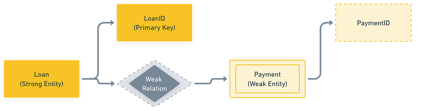
  Example: A Student entity identified by StudentID.

• Weak Entity
  Cannot exist without being linked to a strong entity. It doesn’t have a primary key of its own.
  Example: A Payment entity that only exists if a Loan exists.
  → Denoted with a double rectangle in diagrams.

Strong VS Weak Entity

Attributes

Attributes are the properties that define an entity. They are shown as ovals connected to their entities in ER diagrams.

Types of Attributes:

• Simple: Cannot be divided.
  Example: StudentID, AccountNumber.

• Composite: Can be broken down into sub-parts.
  Example: Name → First Name + Last Name.

• Single-Valued: Holds a single value.
  Example: Email.

• Multi-Valued: Can hold multiple values.
  Example: PhoneNumbers, NomineeNames.

• Derived: Can be derived from other attributes.
  Example: Age derived from DOB.

• Null-Valued: Optional attributes.
  Example: MiddleName (can be NULL).

Type of Attributes

Relationships

A relationship is an association between two or more entities. It’s represented using diamonds in ER diagrams.

Relationship

Types of Relationships:

• Strong Relationship — Professor Entity Teaches Course so here we have strong relationship between Professor and Course entity, both can be uniquely identified by their primary keys.

• Weak Relationship — Loan Processes Payment here payment entity is depended on Loan entity is dependent on Loan entity.

Degree of Relationship:

• Unary (Recursive):
  Same entity related to itself.
  Example: Employee manages Employee.

• Binary:
  Two entities involved.
  Example: Student enrolls in Course.

• Ternary:
  Involves three entities.
  Example: Employee works at Branch on a specific Job.

Example for ternary Relationship

Relationship Constraints

1. Mapping Cardinality

Defines how many instances of an entity relate to instances of another.

• One-to-One (1:1):
  Example: Citizen ↔ AadharCard.

• One-to-Many (1:N):
  Example: Citizen ↔ Vehicle.

• Many-to-One (N:1):
  Example: Course ← Professor.

• Many-to-Many (M:N):
  Example: Customer ↔ Product.

2. Participation Constraints

• Total Participation:
  Means all the entities in entity set are related with some entity. For example — In the diagram shown below Customer borrows a loan, so every loan entities (L1,L2,Ln) under the Entity Set Loan is related with a customer, there won’t be any loan entity that won’t be related to any customer. So, relationship of the loan with Customer is Total Participation like every loan entities will be having some customer that would be paying it.

• Partial Participation:
  Means it’s not necessary that every entities in the entity set is related with some entity. For example, there can be some customers that haven’t borrowed any loan, so they exist as partial participation. So, relationship of the customer is a partial participation with the loan, like not every customer is having some loan.

Partial VS Total Participation

The ER model is a crucial first step in designing a well-structured database. It helps visualize how different pieces of data relate to each other before translating them into tables and schemas in a relational database.

🧠 Final Thoughts

In this second part of our DBMS blog series, we explored some of the most foundational yet crucial concepts — Normalization, Denormalization, and the Entity-Relationship (ER) Model. These concepts not only shape how data is structured and maintained but also influence how efficiently a database performs in real-world applications.

Understanding when to normalize or denormalize data, and how to model entities and their relationships, lays the groundwork for designing robust and scalable databases.

In the upcoming Part 3, we’ll dive deeper into advanced topics like Transactions, Concurrency Control, Indexing, and more. Stay tuned and keep learning — your journey into the world of databases is just getting started!