From Thresholds to Probabilities

In the previous post, we looked at Softmax and NLL loss, both critical for output interpretation and learning in Transformers. Now let’s dive into what happens within the network: activation functions. Specifically, GELU.

---

What is GeLU?

GeLU, or, Gaussian Error Linear Unit can be simply defined as a modified, more flexible version of ReLU. By “soft-gating” rather than hard clamping, GeLU avoids abrupt transitions that can destabilize deep stacks of self-attention layers and Feed-Forward Network layers. Abrupt transitions in ReLU arise when a neuron's input is near zero, causing the output and gradient to become zero — a phenomenon known as the "dying ReLU" problem. This leads to dead neurons and disrupts learning. One way to address this is by introducing noise to the input before applying ReLU.

GeLU can be interpreted as the expected output of a ReLU when its input is corrupted by Gaussian noise. Instead of a hard 0/1 gate like ReLU, GELU smoothly weights inputs by their probability of being significant, effectively allowing more nuanced gradient flow.

---

Deriving and explaining GeLU

We just defined GeLU as the expectation of ReLU applied to input corrupted with Gaussian noise. But what exactly is this Gaussian noise?

Gaussian noise refers to a normal distribution with mean 0 and standard deviation 1. In the context of GeLU, it appears when we compute Φ(x), the cumulative distribution function (CDF) of the standard normal. This value represents the probability that a standard normal variable is less than x essentially quantifying how significant the input x is.

$$\phi(x)=P(ε≤x)$$

$$\phi(x) = \int^x_{-\infty}\frac{1}{\sqrt{2\pi}}e^{\frac{-t^2}{2}}dt$$

where

$$t= \varepsilon \sim N(0,1)$$

Now, we know that ReLU outputs x when it is greater than 1 and 0 when it is less than 1. Therefore, the probability that the neuron is on can be mathematically defined as

$$P(x+\varepsilon>0)$$

$$=P(\varepsilon>-x)$$

Now flip the inequality

$$=1-P(\varepsilon\le-x)$$

since

$$\phi(x)=P(ε≤x)$$

by symmetry of the Gaussian curve

$$P(\varepsilon\le-x) = \phi(-x) \Longrightarrow P(\varepsilon>-x) = 1-\phi(-x)$$

$$P(x+\varepsilon >0) =1-\phi(-x)$$

again, using the symmetry of Gaussian distribution

$$P(x+\varepsilon>0) = 1-(1-\phi(x))$$

$$P(x+\varepsilon >0) =\phi(x)$$

Therefore, the CDF Φ(x), a major component of the function, can be interpreted as the probability that a Gaussian noise ε∼N(0,1) exceeds −x, or equivalently, the probability that the neuron’s perturbed input x+ε is positive.

We are more interested in the latter.

We can also visualise both the interpretations of Φ(x) with the help of this graph:

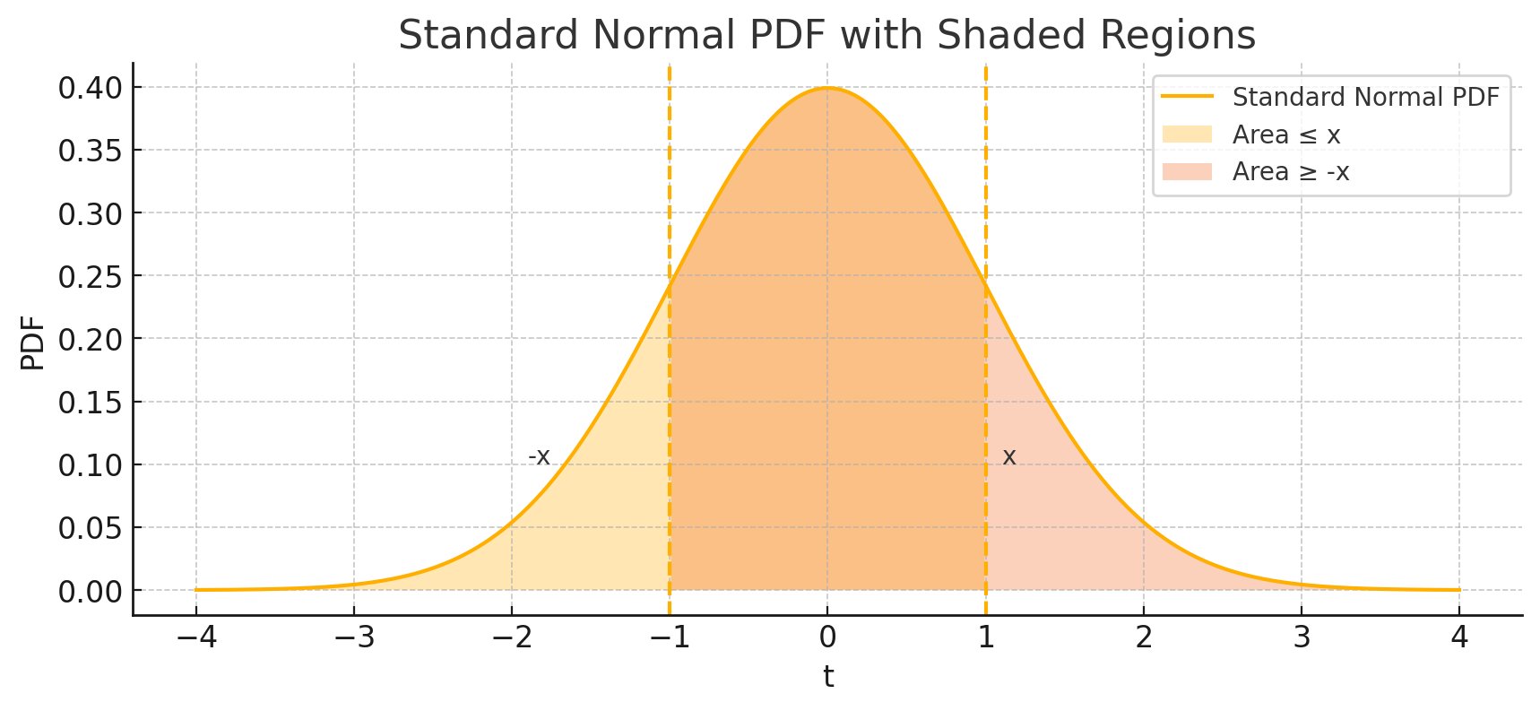
Both Area <= x and Area >= -x means CDF Φ(x).

Now, lets introduce ReLU to our gaussian corrupted input.

$$ReLU = max(0, x+\varepsilon)$$

taking Expectation of ReLU

$$\mathbb{E}[ReLU(x+\varepsilon)]$$

$$=\mathbb{E}[max(0, x+\varepsilon)]$$

Why is this useful?

• For very negative value of x, the perturbed ReLU input samples (x + ɛ) are < 0 meaning the average is approximately 0.

• For very positive value of x, the perturbed ReLU input samples (x + ɛ) are > 0 meaning the average is approximately x itself.

• When x ≈ 0, we get a smooth transition from 0 to x.

$$\therefore \mathbb{E}[max(0,x+ϵ)]=\int^\infty_{-\infty} ​ max(0,x+\varepsilon)⋅p(t)dt$$

after some more math, we get our final equation:

$$\mathbb{E}[max(0, x+\varepsilon)] = x\cdot\phi(x) +\varphi(x)$$

The extra term ϕ(x) (PDF of standard normal at x) is small and disappears fast as x → ±∞. So for efficient computation and very similar performance, Expectation is approximated as:

$$\mathbb{E}[max(0, x+\varepsilon)] \approx x\cdot\phi(x)$$

By our definition of GeLU,

$$GeLU(x) = x\cdot\phi(x)$$

The graph of GeLU(x) is:

That smooth portion near x=0 is due to Φ(x) handling a Standard Normal variable (ε).

To understand how Φ(x) handling a Standard Normal variable (ε) provides a smooth transition, we can look at another Φ(x) graph:

Even when x is 0 or very near to 0, Φ(x) outputs a positive value leading to a very smooth transition instead of a very abrupt, hard-clamped transition which is seen in ReLU.

---

Why is GeLU widely used in modern-day LLMs?

GeLU averages ReLU over all possible small Gaussian jitters meaning the output gradually changes as x moves. This makes it naturally capable of handling noise in data and is less sensitive to tiny changes, i.e, more stable gradients.

It has been observed that models with GeLU converge faster as compared to other activation functions.

---

Approximations and Implementations of GeLU

Although we derived GeLU(x) as x⋅Φ(x), in practice we use a Gaussian error function to define it:

$$GeLU(x) = \frac{1}{2}(1+erf(\frac{x}{\sqrt2}))$$

To make GeLU even more computationally efficient, we use approximations of it. The most used approximation is:

$$GeLU(x) \approx 0.5x(1+tanh[\sqrt\frac{2}{\pi}(x+0.044715x^3)])$$

The sigmoid based approximation is:

$$GeLU(x) \approx x\cdot\sigma(1.702x)$$

---

Gradient of GeLU

We know that

$$GeLU(x) = x\cdot\phi(x)$$

Therefore,

$$\frac{\partial GeLU(x)}{\partial x} =\frac{\partial x\phi(x)}{\partial{x}}$$

$$= \phi(x) + x\cdot\phi^`(x)$$

$$= \phi(x) + x\cdot\varphi(x)$$

Or

$$= \phi(x) + x\cdot p(X=x)$$

where p(X=x) means the value of PDF at x.

---

Conclusion

The Gaussian Error Linear Unit (GeLU) stands out by blending deterministic input with probabilistic reasoning. GeLU offers a compelling balance between mathematical elegance and practical performance making it a popular choice in modern deep learning architectures like Transformers. Unlike ReLU’s hard cutoff, GeLU softly gates inputs based on the likelihood that they remain positive under Gaussian noise. This results in a smoother, more stable activation function that better reflects real-world uncertainty in neural activations.