Decoding Autoencoders: From Theory to Implementation
 Shaun Liew
As I delved into the fascinating world of image generation and manipulation, I encountered autoencoders - a fundamental building block that bridges the gap between understanding and generating visual content. Let me share what I've learned about these remarkable neural networks and why they're so crucial in modern AI visual generation.
What Are Autoencoders?

At its core, an autoencoder is like a digital compression artist. Imagine you have a massive collection of Pokémon cards, and you want to create a compact storage system. You'd identify the essential features that make each Pokémon unique - their type, color patterns, and distinctive characteristics - and store just those key elements. Later, you could use this compressed information to recreate the original cards. That's essentially what an autoencoder does with data.
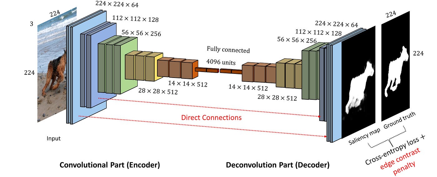
An autoencoder consists of two main components working in tandem:

The Encoder: This network compresses input data into a lower-dimensional representation called the "latent space" or "bottleneck layer." Think of it as extracting the DNA of your data - capturing the most essential features while discarding redundant information.
The Decoder: This network takes the compressed representation and attempts to reconstruct the original input. It's like a skilled artist who can recreate a full painting from just a few key sketches.
The magic happens in the bottleneck layer - a compressed representation that forces the network to learn only the most important features of the input data. This constraint is what makes autoencoders so powerful for learning meaningful representations.
The Learning Process
Autoencoders learn through a simple yet elegant objective: minimize the reconstruction error. The mathematical representation is:
$$L(\theta, \phi) = \frac{1}{n} \sum_{i=1}^{n} \left( \mathbf{x}^{(i)} - f_\theta\left(g_\phi\left(\mathbf{x}^{(i)}\right)\right) \right)^2$$
Where:
gϕ represents the encoder function
fθ represents the decoder function
The goal is to make the reconstructed output x' as close as possible to the original input x
This reconstruction loss encourages the network to capture the essential patterns in the data while learning a compact representation.
Why Autoencoders Matter

During my learning journey, I discovered several key applications that make autoencoders invaluable:
Dimensionality Reduction: Unlike traditional methods like PCA, autoencoders can capture non-linear relationships in data, making them more powerful for complex datasets.
Feature Learning: The bottleneck layer learns meaningful representations that can be used for other tasks like classification or clustering.
Data Compression: They provide a learned compression scheme tailored to specific types of data.
Anomaly Detection: By learning to reconstruct normal data well, they struggle with unusual patterns, making them excellent for detecting outliers.
The Bottleneck: Where Magic Happens
The size of the bottleneck layer (compressed representation) is crucial. From my experiments, I learned that:
Too small: The network struggles to capture enough information, leading to blurry reconstructions
Too large: The network might just memorize the data without learning meaningful patterns
Just right: The network learns compact, meaningful representations
Through my hands-on experience, I observed that as I increased the bottleneck size from 2 to 50 dimensions, the reconstructed images became progressively clearer and more detailed.
Vanilla Autoencoders: The Foundation
Basic autoencoders use fully connected layers and work well for simpler data. However, when I started working with images, I quickly realized their limitations. Flattening a 28×28 image into 784 individual pixels loses the spatial relationships that make images meaningful. This is where convolutional autoencoders come to the rescue.
Convolutional Autoencoders: Spatial Awareness
Convolutional autoencoders represent a significant evolution in the autoencoder family. Instead of treating images as flat vectors, they preserve and leverage spatial relationships through convolutional layers.
Key Advantages:
Spatial Preservation: Convolutional layers maintain the 2D structure of images, allowing the network to understand local patterns and relationships.
Parameter Efficiency: Shared weights in convolutional layers mean fewer parameters compared to fully connected networks, reducing overfitting risk.
Translation Invariance: The network can recognize patterns regardless of their position in the image.
Architecture Design:
In the encoder, convolutional layers with stride > 1 or pooling operations progressively reduce spatial dimensions while increasing the number of feature maps. The decoder reverses this process using transposed convolutions (also called deconvolutions) or upsampling operations.
A typical progression might look like:
Input: 28×28×1 → Conv → 14×14×32 → Conv → 7×7×64 → Conv → 4×4×128 (Encoder)
4×4×128 → TransConv → 7×7×64 → TransConv → 14×14×32 → TransConv → 28×28×1 (Decoder)
Visualizing Similarity: The Power of Learned Representations
One of the most exciting discoveries in my learning journey was using t-SNE to visualize the learned representations. When I projected the bottleneck layer activations into 2D space, I found that similar images naturally clustered together. Images of the same digit formed distinct groups, validating that the autoencoder had learned meaningful representations of the data.
This clustering behavior is incredibly valuable because it means:
Similar images have similar encoded representations
The latent space has semantic meaning
We can navigate the space to find related content
Limitations and Considerations
Through my experiments, I also learned about some important limitations:
Quality vs. Compression Trade-off: Smaller bottlenecks mean more compression but potentially lower quality reconstructions.
Limited Generative Capability: Basic autoencoders aren't great at generating entirely new content - they're optimized for reconstruction, not creation.
Mode Collapse: Sometimes the network learns to ignore certain types of input variations.
Hands-On Implementation: Building Autoencoders from the Project Code
Now that we've covered the theory, let's dive into the practical implementation using the code from my project knowledge. I'll walk you through the actual implementation with detailed code explanations, sharing the insights and observations I made during the process.
Setting Up the Environment
First, let's look at how the environment was set up in the project:
# Install torch_snippets - a utility library for PyTorch that simplifies common operations
!pip install -q torch_snippets

# Import necessary libraries
from torch_snippets import *           # Contains helpful utilities for training and visualization
from torchvision.datasets import MNIST # Pre-built MNIST dataset loader
from torchvision import transforms     # Image transformation utilities
device = 'cuda' if torch.cuda.is_available() else 'cpu'  # Use GPU if available
Key Observation: The project uses torch_snippets, which is a helpful utility library that simplifies many common PyTorch operations and provides convenient functions for visualization and training.
Data Preparation
The data preparation follows a standard approach for MNIST:
# Define image transformations that will be applied to each image
img_transform = transforms.Compose([
    transforms.ToTensor(),              # Convert PIL image to tensor (0-255 → 0-1)
    transforms.Normalize([0.5], [0.5]), # Normalize to [-1, 1]: (x - 0.5) / 0.5
    transforms.Lambda(lambda x: x.to(device)) # Move tensor to GPU/CPU automatically
])

# Load training and validation datasets
# MNIST contains 28x28 grayscale images of handwritten digits (0-9)
trn_ds = MNIST('/content/', transform=img_transform, train=True, download=True)
val_ds = MNIST('/content/', transform=img_transform, train=False, download=True)

# Create data loaders for batch processing
batch_size = 256  # Process 256 images at once for efficient GPU utilization
trn_dl = DataLoader(trn_ds, batch_size=batch_size, shuffle=True)   # Shuffle training data
val_dl = DataLoader(val_ds, batch_size=batch_size, shuffle=False)  # Don't shuffle validation
Important Design Choice: Notice the normalization to [-1, 1] range using Normalize([0.5], [0.5]). This centers the data around zero, which often leads to better training stability. The Lambda function automatically moves data to the appropriate device (CPU/GPU).
Vanilla Autoencoder Implementation
Here's the actual vanilla autoencoder implementation from the project with detailed explanations:
class AutoEncoder(nn.Module):
    def __init__(self, latent_dim):
        super().__init__()
        self.latend_dim = latent_dim  # Store the latent dimension size

        # ENCODER: Progressively compress 784 pixels down to latent_dim values
        # This learns to extract the most important features from the input
        self.encoder = nn.Sequential(
            # First compression: 784 → 128 (reduce by ~6x)
            nn.Linear(28 * 28, 128),  # 28x28 = 784 flattened pixels as input
            nn.ReLU(True),            # ReLU activation (inplace=True for memory efficiency)

            # Second compression: 128 → 64 (reduce by 2x)
            nn.Linear(128, 64),
            nn.ReLU(True),

            # Final compression: 64 → latent_dim (the bottleneck!)
            # This is where the magic happens - all image info compressed to latent_dim numbers
            nn.Linear(64, latent_dim)  # No activation here - let values be any real number
        )

        # DECODER: Progressively expand latent_dim back to 784 pixels
        # This learns to reconstruct the original image from compressed representation
        self.decoder = nn.Sequential(
            # First expansion: latent_dim → 64
            nn.Linear(latent_dim, 64),
            nn.ReLU(True),            # ReLU helps learn non-linear reconstruction

            # Second expansion: 64 → 128
            nn.Linear(64, 128),
            nn.ReLU(True),

            # Final expansion: 128 → 784 (back to original size)
            nn.Linear(128, 28 * 28),
            nn.Tanh()  # Tanh outputs [-1,1] to match our normalized input range
        )

    def forward(self, x):
        # x shape: (batch_size, 1, 28, 28) - batch of grayscale images

        # STEP 1: Flatten images from 2D to 1D
        # Convert (batch_size, 1, 28, 28) → (batch_size, 784)
        x = x.view(len(x), -1)  # -1 means "figure out this dimension automatically"

        # STEP 2: Encode - compress to latent representation
        x = self.encoder(x)     # Now x has shape (batch_size, latent_dim)

        # STEP 3: Decode - reconstruct from latent representation
        x = self.decoder(x)     # Now x has shape (batch_size, 784)

        # STEP 4: Reshape back to image format for visualization/loss calculation
        # Convert (batch_size, 784) → (batch_size, 1, 28, 28)
        x = x.view(len(x), 1, 28, 28)

        return x  # Reconstructed images
Architecture Deep Dive:
Why this Layer Structure?: The symmetric design (784→128→64→latent_dim→64→128→784) ensures the decoder can "reverse" what the encoder learned. Each layer halves or doubles the dimensions systematically.
The Bottleneck Magic: The
latent_dimlayer is where all 784 pixels worth of information gets compressed. Iflatent_dim=3, we're forcing the network to represent entire handwritten digits with just 3 numbers!Activation Functions:
ReLU in hidden layers: Allows learning complex non-linear patterns
No activation in encoder output: Latent values can be any real numbers
Tanh in decoder output: Ensures outputs match our [-1,1] input range
Information Flow: Input → Compress → Bottleneck → Expand → Reconstruction
Training and Validation Functions
The project includes clean, well-structured training functions with detailed explanations:
def train_batch(input, model, criterion, optimizer):
    """
    Train the model on one batch of data

    Args:
        input: Batch of input images
        model: The autoencoder model
        criterion: Loss function (measures reconstruction quality)
        optimizer: Updates model weights based on gradients
    """
    model.train()          # Set model to training mode (enables dropout, batch norm, etc.)
    optimizer.zero_grad()  # Clear gradients from previous batch

    # Forward pass: get reconstructed images
    output = model(input)  # input → encoder → decoder → output

    # Calculate loss: how different is output from input?
    # This is the KEY insight: we want output ≈ input (perfect reconstruction)
    loss = criterion(output, input)

    # Backward pass: calculate gradients
    loss.backward()        # Compute ∂loss/∂weights for all parameters

    # Update weights: move in direction that reduces loss
    optimizer.step()       # weights = weights - learning_rate * gradients

    return loss

@torch.no_grad()  # Disable gradient computation for efficiency
def validate_batch(input, model, criterion):
    """
    Evaluate model on validation data (no weight updates)
    """
    model.eval()          # Set to evaluation mode (disables dropout, etc.)
    output = model(input) # Get reconstructions
    loss = criterion(output, input)  # Measure reconstruction quality
    return loss
Critical Observation: The loss function compares the model output directly with the input - this is the essence of autoencoder training. We're teaching the network to be an "identity function" but forced through a narrow bottleneck, which makes it learn meaningful compression.
Model Architecture Analysis
Let's examine the model summary that was generated:
# Import library for model architecture visualization
from torchsummary import summary

# Create a model with 3-dimensional latent space (very compressed!)
model = AutoEncoder(3).to(device)

# Show detailed architecture info: layers, output shapes, parameter counts
summary(model, torch.zeros(2,1,28,28))  # Use dummy input to trace shapes
The summary revealed crucial insights about our 3-dimensional latent space model:
Layer (type:depth-idx)                Output Shape              Param #
============================================================================
├─Sequential: 1-1                     [-1, 3]                   --
│    └─Linear: 2-1                    [-1, 128]                 100,480  # 784*128 + 128 bias
│    └─ReLU: 2-2                      [-1, 128]                 --
│    └─Linear: 2-3                    [-1, 64]                  8,256    # 128*64 + 64 bias
│    └─ReLU: 2-4                      [-1, 64]                  --
│    └─Linear: 2-5                    [-1, 3]                   195      # 64*3 + 3 bias ← BOTTLENECK!
├─Sequential: 1-2                     [-1, 784]                 --
│    └─Linear: 2-6                    [-1, 64]                  256      # 3*64 + 64 bias
│    └─ReLU: 2-7                      [-1, 64]                  --
│    └─Linear: 2-8                    [-1, 128]                 8,320    # 64*128 + 128 bias
│    └─ReLU: 2-9                      [-1, 128]                 --
│    └─Linear: 2-10                   [-1, 784]                 101,136  # 128*784 + 784 bias
│    └─Tanh: 2-11                     [-1, 784]                 --
============================================================================
Total params: 218,643
Key Insights:
Bottleneck layer (Linear: 2-5): Only 195 parameters but represents the entire image!
Most parameters: In layers connecting to/from the flattened image (784 dimensions)
Parameter efficiency: The bottleneck forces efficient representation learning
Training Process
# Initialize model, loss function, and optimizer
model = AutoEncoder(3).to(device)  # 3D latent space - extreme compression!
criterion = nn.MSELoss()           # Mean Squared Error: measures pixel-wise differences
optimizer = torch.optim.AdamW(     # AdamW: Adam with weight decay (prevents overfitting)
    model.parameters(),
    lr=0.001,        # Learning rate: how big steps to take during optimization
    weight_decay=1e-5 # L2 regularization: keeps weights small
)

num_epochs = 5
log = Report(num_epochs)  # torch_snippets utility for tracking training progress

for epoch in range(num_epochs):
    # TRAINING PHASE: Update model weights
    N = len(trn_dl)  # Number of batches in training set
    for ix, (data, _) in enumerate(trn_dl):  # Note: we ignore labels (unsupervised!)
        loss = train_batch(data, model, criterion, optimizer)
        # Record progress: position in training, loss value
        log.record(pos=(epoch + (ix+1)/N), trn_loss=loss, end='\r')

    # VALIDATION PHASE: Check performance without updating weights
    N = len(val_dl)
    for ix, (data, _) in enumerate(val_dl):
        loss = validate_batch(data, model, criterion)
        log.record(pos=(epoch + (ix+1)/N), val_loss=loss, end='\r')

    log.report_avgs(epoch+1)  # Print average losses for this epoch

# Plot training curves to visualize learning progress
log.plot_epochs(log=True)  # Log scale often shows trends better
Training Observations:

Unsupervised Learning: Notice we ignore the labels
_- autoencoders learn from images alone!Loss Convergence: Both training and validation losses decreased smoothly
No Overfitting: Training and validation losses stayed close together
Quick Convergence: Major improvements in first few epochs, then diminishing returns
Visualizing Results
The project includes excellent visualization code to see what the network learned:
# Test the trained model on some validation examples
for _ in range(3):  # Show 3 random examples
    # Pick a random image from validation set
    ix = np.random.randint(len(val_ds))
    im, _ = val_ds[ix]  # Get image (ignore label)

    # Get reconstruction: add batch dimension [1, 28, 28] → [1, 1, 28, 28]
    _im = model(im[None])[0]  # [None] adds batch dimension, [0] removes it

    # Create side-by-side comparison
    fig, ax = plt.subplots(1, 2, figsize=(3,3))
    show(im[0], ax=ax[0], title='input')      # Original image
    show(_im[0], ax=ax[1], title='prediction') # Reconstructed image
    plt.tight_layout()
    plt.show()
Visual Results with 3D Latent Space:


✅ Recognizable: Could identify which digit it was supposed to be
❌ Blurry: Fine details were lost due to extreme compression
🤔 Trade-off visible: 784 pixels → 3 numbers → 784 pixels is lossy compression
Experimenting with Different Latent Dimensions
One of the most illuminating experiments was comparing different bottleneck sizes. The project tested latent dimensions of 2, 3, 5, 10, and 50:
def train_aec(latent_dim):
    model = AutoEncoder(latent_dim).to(device)
    criterion = nn.MSELoss()
    optimizer = torch.optim.AdamW(model.parameters(), lr=0.001, weight_decay=1e-5)

    num_epochs = 5
    log = Report(num_epochs)

    for epoch in range(num_epochs):
        N = len(trn_dl)
        for ix, (data, _) in enumerate(trn_dl):
            loss = train_batch(data, model, criterion, optimizer)
            log.record(pos=(epoch + (ix+1)/N), trn_loss=loss, end='\r')

        N = len(val_dl)
        for ix, (data, _) in enumerate(val_dl):
            loss = validate_batch(data, model, criterion)
            log.record(pos=(epoch + (ix+1)/N), val_loss=loss, end='\r')
        log.report_avgs(epoch+1)
    log.plot(log=True)
    return model

aecs = [train_aec(dim) for dim in [50, 2, 3, 5, 10]]

for _ in range(10):
    ix = np.random.randint(len(val_ds))
    im, _ = val_ds[ix]
    fig, ax = plt.subplots(1, len(aecs)+1, figsize=(10,4))
    ax = iter(ax.flat)
    show(im[0], ax=next(ax), title='input')
    for model in aecs:
        _im = model(im[None])[0]
        show(_im[0], ax=next(ax), title=f'prediction\nlatent-dim:{model.latend_dim}')
    plt.tight_layout()
    plt.show()


Key Findings:
Latent dim 2: Barely recognizable digit shapes, extreme blur
Latent dim 3: Recognizable digits but significant blur
Latent dim 5: Clearer shapes, better digit recognition
Latent dim 10: Good balance of compression (98.7% reduction) and quality
Latent dim 50: Very clear reconstructions, but less impressive compression (93.6% reduction)


The Compression Math:
Original: 784 pixels
3D latent: 784 → 3 (99.6% compression!)
10D latent: 784 → 10 (98.7% compression)
50D latent: 784 → 50 (93.6% compression)
Convolutional Autoencoder Implementation
The project then moves to a more sophisticated approach that respects the spatial nature of images:
class ConvAutoEncoder(nn.Module):
    def __init__(self):
        super().__init__()

        # ENCODER: Preserve spatial relationships while compressing
        # Key idea: Use convolutions instead of flattening immediately
        self.encoder = nn.Sequential(
            # Layer 1: 28x28x1 → 10x10x32
            nn.Conv2d(1, 32, 3, stride=3, padding=1),  # Convolve with 32 filters
            nn.ReLU(True),                             # Non-linearity
            nn.MaxPool2d(2, stride=2),                 # Downsample: 10x10 → 5x5

            # Layer 2: 5x5x32 → 3x3x64
            nn.Conv2d(32, 64, 3, stride=2, padding=1), # More filters, smaller spatial size
            nn.ReLU(True),
            nn.MaxPool2d(2, stride=1)                  # Final spatial reduction: 3x3 → 2x2

            # Final bottleneck: 2x2x64 = 256 dimensional representation
            # Much larger than 3D, but preserves spatial structure!
        )

        # DECODER: Reconstruct spatial dimensions using transposed convolutions
        # These are like "reverse convolutions" that upsample feature maps
        self.decoder = nn.Sequential(
            # Layer 1: 2x2x64 → 5x5x32
            nn.ConvTranspose2d(64, 32, 3, stride=2),    # "Deconvolution" - upsamples
            nn.ReLU(True),

            # Layer 2: 5x5x32 → 15x15x16
            nn.ConvTranspose2d(32, 16, 5, stride=3, padding=1),  # Larger upsampling
            nn.ReLU(True),

            # Layer 3: 15x15x16 → 28x28x1 (back to original size!)
            nn.ConvTranspose2d(16, 1, 2, stride=2, padding=1),   # Single channel output
            nn.Tanh()  # Output range [-1, 1] to match input normalization
        )

    def forward(self, x):
        # x shape: (batch_size, 1, 28, 28) - keep spatial structure!

        # Encode: preserve spatial relationships while compressing
        x = self.encoder(x)  # → (batch_size, 64, 2, 2)

        # Decode: reconstruct spatial structure
        x = self.decoder(x)  # → (batch_size, 1, 28, 28)

        return x  # Reconstructed images with spatial structure preserved

Revolutionary Improvements:
Spatial Awareness: Instead of flattening to 784 numbers, we maintain 2D structure throughout
Local Pattern Recognition: Convolutions detect local features (edges, curves) that make up digits
Translation Invariance: A "7" is recognized as a "7" regardless of position in the image
Parameter Efficiency: Shared convolutional weights vs. unique fully-connected weights
Architecture Progression:
Encoder: 28×28×1 → 10×10×32 → 5×5×32 → 3×3×64 → 2×2×64
Decoder: 2×2×64 → 5×5×32 → 15×15×16 → 28×28×1
Bottleneck Comparison:
Vanilla: 3 numbers (extreme compression, spatial info lost)
Convolutional: 2×2×64 = 256 numbers (moderate compression, spatial info preserved)
Convolutional Autoencoder Results
The training process was identical, but the results were dramatically different:


Model Summary Insights:
Total parameters: 50,161 (much fewer than vanilla!)
Bottleneck: MaxPool2d-6 layer with shape (batch_size, 64, 2, 2)
Efficiency: Fewer parameters but better performance due to spatial awareness
Performance Comparison:
Vanilla (3D): Blurry, recognizable but lacking detail
Convolutional: Sharp, clear reconstructions with preserved spatial relationships
Understanding t-SNE: Visualizing High-Dimensional Latent Spaces
One of the important use case of AutoEncoder is that we can cluster the similar images together using the latent space given that similar images have similar representation.
One of the most fascinating experiments was visualizing the learned representations using t-SNE (t-Distributed Stochastic Neighbor Embedding). Let me explain what t-SNE is and why it's so powerful:
What is t-SNE?
t-SNE is a dimensionality reduction technique specifically designed for visualization. Think of it as a smart way to create a 2D map of high-dimensional data while preserving the "neighborhoods" - similar points stay close together, dissimilar points are pushed apart.
The Challenge: Our autoencoder creates representations in high-dimensional spaces (64×2×2 = 256 dimensions for conv autoencoder). Humans can't visualize 256-dimensional space!
The Solution: t-SNE "flattens" this 256D space down to 2D while trying to keep similar images close together and different images far apart.
How t-SNE Works (Conceptually)
Imagine you have a crowd of people in a large room, and you want to create a map of their relationships:
Step 1: Measure how "similar" each person is to every other person (in our case, how similar each image's latent representation is)
Step 2: Create a 2D map where people who are similar in the high-dimensional space are placed close together
Step 3: Iteratively adjust positions to best preserve these similarity relationships
The t-SNE Visualization Code
# Extract latent representations for all validation images
latent_vectors = []  # Will store encoded representations
classes = []         # Will store true digit labels (for coloring)

# Process all validation data
for im, clss in val_dl:  # im=images, clss=class labels
    # Get latent representation from encoder
    latent_rep = model.encoder(im)  # Shape: (batch_size, 64, 2, 2) for conv autoencoder

    # Flatten spatial dimensions: (batch_size, 64, 2, 2) → (batch_size, 256)
    latent_rep = latent_rep.view(len(im), -1)  # -1 means "calculate this dimension"

    latent_vectors.append(latent_rep)  # Add to our collection
    classes.extend(clss)               # Add corresponding labels

# Combine all latent vectors into one big array
latent_vectors = torch.cat(latent_vectors).cpu().detach().numpy()
# Final shape: (10000, 256) - 10,000 validation images, each with 256-dim representation

print(f"Latent vectors shape: {latent_vectors.shape}")
print(f"Classes shape: {len(classes)}")

# Apply t-SNE: 256 dimensions → 2 dimensions
from sklearn.manifold import TSNE
tsne = TSNE(n_components=2)  # Reduce to 2D for visualization
clustered = tsne.fit_transform(latent_vectors)  # This takes a few minutes!

# clustered shape: (10000, 2) - each image now has (x, y) coordinates

# Create the visualization
fig = plt.figure(figsize=(12,10))
cmap = plt.get_cmap('Spectral', 10)  # Color map with 10 colors (for 10 digits)

# Plot each point, colored by its true digit label
plt.scatter(*zip(*clustered), c=classes, cmap=cmap)
plt.colorbar(drawedges=True)
plt.title('t-SNE visualization of learned latent representations')
plt.xlabel('t-SNE Dimension 1')
plt.ylabel('t-SNE Dimension 2')
plt.show()
What the t-SNE Plot Reveals

Amazing Discovery: When you look at the t-SNE plot, you see distinct clusters of colors! Each color represents a different digit (0-9), and similar digits are grouped together spatially.
Why This is Mind-Blowing:
Unsupervised Learning: The autoencoder was NEVER told what digit each image contained
Semantic Organization: Yet it learned to group similar digits together in latent space
Meaningful Representations: The compressed representations capture semantic meaning, not just pixel patterns
What Each Cluster Tells Us:
Tight clusters: Digits that are very consistent (like "1" - simple vertical line)
Spread clusters: Digits with more variation (like "2" - many ways to write it)
Nearby clusters: Digits that share visual features (like "6" and "9" - similar curves)
Distant clusters: Very different digits (like "1" and "8" - completely different shapes)
Why t-SNE Visualization Matters
Validation of Learning: Proves the autoencoder learned meaningful patterns, not just memorization
Debugging Tool: If clusters look random, something's wrong with your model
Feature Quality: Tight, well-separated clusters indicate high-quality learned features
Interpretability: Helps us understand what the "black box" neural network actually learned
Real-World Applications:
Anomaly Detection: Points far from any cluster might be anomalies
Data Organization: Automatically group similar items without labels
Quality Control: Identify mislabeled data (points in the wrong cluster)
Convolutional vs Vanilla: Side-by-Side Comparison
Here's what I observed when comparing the two approaches:
Performance Comparison:
| Metric | Vanilla (3D) | Convolutional |
| Image Quality | Blurry, recognizable | Sharp, detailed |
| Parameter Count | 218,643 | 50,161 |
| Training Speed | Slower | Faster |
| Spatial Structure | Lost | Preserved |
| Compression Ratio | 99.6% | 67.3% |
| Best Use Case | Extreme compression | Image processing |
Key Observations and Insights
Through working with this code, I gained several crucial insights:
1. Architecture Design Philosophy
# Vanilla: Treats images as vectors of independent pixels
x = x.view(len(x), -1)  # Destroys spatial relationships

# Convolutional: Respects spatial structure of images
# (no flattening until absolutely necessary)
2. The Bottleneck's Role
The bottleneck isn't just compression - it's forced feature learning:
Too small: Information bottleneck forces lossy compression
Too large: Model might just memorize without learning patterns
Just right: Model learns meaningful, generalizable features
3. Loss Function Insight
loss = criterion(output, input) # The key insight!
This simple line encodes a profound idea: learn representations by trying to reconstruct perfectly. The bottleneck constraint forces the model to discover the essential patterns.
4. Unsupervised Learning Power
The t-SNE visualization proved that autoencoders discover semantic structure without any labels - they learn what makes digits similar or different just from trying to reconstruct them!
5. Practical Implementation Details
Normalization Matters:
transforms.Normalize([0.5], [0.5])  # Maps [0,1] to [-1,1]
nn.Tanh()  # Output range [-1,1] matches input
Device Management:
transforms.Lambda(lambda x: x.to(device)) # Auto-GPU transfer
Memory Efficiency:
nn.ReLU(True)  # inplace=True saves memory
@torch.no_grad()  # Disable gradients during validation
This hands-on experience with the project code provided deep intuition about how autoencoders work in practice, revealing both their elegant simplicity and hidden complexity through real implementation details and experimental results.
Reference:
https://www.datacamp.com/tutorial/introduction-to-autoencoders
https://github.com/PacktPublishing/Modern-Computer-Vision-with-PyTorch-2E?tab=readme-ov-file
Subscribe to my newsletter
Read articles from Shaun Liew directly inside your inbox. Subscribe to the newsletter, and don't miss out.
Written by
Shaun Liew
Shaun Liew
Year 3 Computer Sciences Student from Universiti Sains Malaysia. Keep Learning.