From Noise to Images: Mastering Variational Autoencoders
 Shaun Liew
From Autoencoders to Variational Autoencoders: Solving the Generation Problem
In my previous exploration of autoencoders, I discovered their remarkable ability to learn compressed representations of data and reconstruct images with impressive fidelity. However, as I delved deeper into generative modeling, I encountered a fundamental limitation that led me to an exciting evolution: Variational Autoencoders (VAEs).
The Generation Problem: When Autoencoders Fall Short
After successfully training my convolutional autoencoder on MNIST digits, I was curious about its generative capabilities. The latent space seemed to capture meaningful representations - similar digits clustered together beautifully in my t-SNE visualizations. But what would happen if I tried to generate completely new images by sampling random points from this learned latent space?
The Random Sampling Experiment
I decided to test this by extracting the statistical properties of the learned latent space and generating random vectors based on these statistics:
# Extract latent representations from all validation images
latent_vectors = []
classes = []
for im, clss in val_dl:
    latent_vectors.append(model.encoder(im))
    classes.extend(clss)

# Reshape to analyze the distribution
latent_vectors = torch.cat(latent_vectors).cpu().detach().numpy().reshape(10000, -1)

# Generate random vectors based on learned statistics
rand_vectors = []
for col in latent_vectors.transpose(1,0):
    mu, sigma = col.mean(), col.std()  # Extract mean and std for each dimension
    rand_vectors.append(sigma*torch.randn(1,100) + mu)  # Sample from Gaussian

# Generate images from these random vectors
rand_vectors = torch.cat(rand_vectors).transpose(1,0).to(device)
fig, ax = plt.subplots(10,10,figsize=(7,7)); ax = iter(ax.flat)
for p in rand_vectors:
    img = model.decoder(p.reshape(1,64,2,2)).view(28,28)
    show(img, ax=next(ax))
The Disappointing Results

The results were... disappointing. Instead of generating recognizable digits, I got a grid of blurry, nonsensical images that barely resembled anything meaningful. The generated "digits" looked like random noise shaped vaguely like numbers - far from the crisp, clear digits I had hoped to create.
Why did this happen? The problem lies in how traditional autoencoders learn their latent representations:
Sparse Coverage: The autoencoder only learns to represent the specific training examples it has seen. Large regions of the latent space remain "unexplored" and don't correspond to valid data.
No Distribution Guarantee: There's no guarantee that the latent space follows any particular distribution. Random sampling from statistical properties doesn't ensure we're sampling from regions that decode to meaningful images.
Overfitting to Data Points: The model learns to map specific inputs to specific latent points, but doesn't learn a continuous, smooth mapping that would enable generation.
This limitation revealed a fundamental issue: traditional autoencoders are optimized for reconstruction, not generation. They're excellent at compressing and reconstructing known data, but poor at creating new, realistic samples.
Enter Variational Autoencoders: A Probabilistic Solution

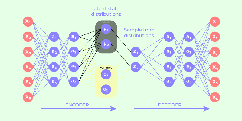
This is where Variational Autoencoders (VAEs) came to my rescue. VAEs address the generation problem by fundamentally reimagining how we think about the latent space - transforming it from a collection of fixed points to a structured probability distribution.
Understanding the Latent Space
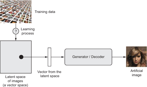
Before diving into VAEs, I needed to clarify what the latent space actually represents. I learned to think of the latent space as a compressed "DNA blueprint" of data. Just as DNA contains the essential genetic information needed to construct a living organism, the latent space contains the essential features needed to reconstruct (or generate) data.
In the context of images:
High-dimensional input: A 28×28 MNIST image has 784 pixel values
Low-dimensional latent space: Compressed to perhaps 20 key numbers that capture essential features (curves, lines, angles)
Meaningful representation: These 20 numbers encode concepts like "roundness," "vertical lines," "loops," etc.
The magic happens when this latent space is structured - meaning similar concepts are positioned close together, enabling smooth transitions and meaningful interpolations.
The Probabilistic Revolution

The fundamental insight of VAEs is brilliantly simple yet profound: instead of mapping each input to a single fixed point in latent space, map it to a probability distribution over that space.
Let me break this down with a concrete example:
Traditional Autoencoder Flow:
Pikachu Image → Encoder → Fixed Vector [1.2, -0.5, 0.8] → Decoder → Same Pikachu
VAE Flow:
Pikachu Image → Encoder → Distribution Parameters:
                         ├─ μ (mean): [1.2, -0.5, 0.8]
                         └─ σ (std): [0.3, 0.2, 0.4]
                      → Sample z from N(μ, σ²) → Decoder → Pikachu Variant
This was my "aha!" moment: the encoder now outputs two vectors instead of one:
μ (mu): The mean vector representing the "center" of Pikachu features
σ (sigma): The standard deviation vector representing the "spread" or variation around that center
The Mathematics Behind VAE: Understanding KL Divergence
Why Probabilistic Encoding?
As I studied VAEs deeper, I realized the shift to probabilistic encoding solves several critical problems:
Enables Variation: By sampling from the distribution, we get different latent vectors each time, creating natural variations
Smooth Latent Space: Forces the model to learn continuous representations rather than isolated points
Principled Generation: Provides a mathematical framework for ensuring that random sampling produces meaningful outputs
The Gaussian Choice: Why N(0,1)?
VAEs typically model the latent distribution as a Gaussian (normal) distribution. But why Gaussian, and why specifically N(0,1)?
Why Gaussian?
Mathematical convenience: Gaussian distributions have well-known properties and are easy to work with
Central Limit Theorem: Many natural phenomena are approximately Gaussian
Reparameterization: Allows for the crucial "reparameterization trick" I'll discuss next
Why N(0,1) specifically?
Standardization: Centers the latent space around zero with unit variance
Numerical stability: Prevents extreme values that could destabilize training
Universal sampling: Makes generation simple - just sample from standard normal distribution
The Sampling Step: Reparameterization Trick
Here's where I encountered the mathematical elegance of VAEs. The sampling process uses the reparameterization trick:
$$z = \mu + \sigma \odot \epsilon$$
Where:
μ: Learned mean vector (location parameter)
σ: Learned standard deviation vector (scale parameter)
ε: Random noise sampled from N(0,1)
⊙: Element-wise multiplication
z: Final latent vector used for reconstruction/generation
Why this formulation?
Differentiability: The randomness is moved to ε, making the operation differentiable with respect to μ and σ
Controlled randomness: We can control the amount and direction of variation through learned parameters
Training stability: Gradients can flow through μ and σ during backpropagation
Understanding KL Divergence
The Kullback-Leibler (KL) divergence is what I discovered to be the secret sauce that makes VAEs work for generation. But what exactly is it?
Conceptually: KL divergence measures "how different" two probability distributions are from each other. I learned to think of it as the "distance" between distributions.
In VAE context: We want our learned distributions q(z|x) to be close to a standard normal distribution p(z) = N(0,1).
The mathematical formula for KL divergence between our learned Gaussian and the standard normal is:
$$\text{KL}[q(z|x) || p(z)] = \frac{1}{2} \sum_{i=1}^{d} \left( \mu_i^2 + \sigma_i^2 - \log(\sigma_i^2) - 1 \right)$$
Where:
μᵢ: The i-th dimension of the mean vector
σᵢ²: The i-th dimension of the variance vector
d: Dimensionality of latent space
Why use log-variance instead of variance? In practice, we often predict log(σ²) instead of σ² directly because:
Numerical stability: Prevents σ² from becoming negative
Easier optimization: log-space often behaves better during training
Unbounded range: log(σ²) can be any real number
Breaking Down the KL Loss
I found it helpful to understand what each term in the KL divergence formula does:
μᵢ²: Penalizes means far from 0 (pulls distributions toward origin)
σᵢ²: Penalizes large variances (prevents distributions from becoming too spread out)
-log(σᵢ²): Penalizes small variances (prevents distributions from collapsing to points)
-1: Normalization constant
The beautiful balance: The KL loss creates a "Goldilocks zone" where distributions are:
Not too tight (would lose variation ability)
Not too spread (would lose meaningful structure)
Centered around origin (enables universal generation)
The Complete VAE Flow: Putting It All Together
As I worked through implementing VAEs, I realized the complete flow follows this pattern:
Training Phase:
1. Input: Pikachu image [28×28 pixels]
   ↓
2. Encoder: Compresses to latent space parameters
   ├─ μ: [1.2, -0.5, 0.8] (center of Pikachu features)
   └─ log(σ²): [-0.1, 0.2, -0.3] (spread of variations)
   ↓
3. Sampling: z = μ + σ * ε (where ε ~ N(0,1))
   Result: z = [1.15, -0.48, 0.85] (a Pikachu variant in latent space)
   ↓
4. Decoder: Reconstructs image from z
   Result: Pikachu-like image (similar but not identical)
   ↓
5. Loss Calculation:
   ├─ Reconstruction Loss: MSE(output, input)
   └─ KL Divergence Loss: Forces distributions toward N(0,1)
Generation Phase:
1. Sample: z ~ N(0,1) [random noise]
   ↓
2. Decoder: Generates image from random z
   ↓
3. Result: Brand new Pokémon-like image!
The Two-Component Loss Function
Through my experiments, I confirmed that VAEs optimize a combination of two losses:
1. Reconstruction Loss (MSE)
Purpose: Ensure the model can still reconstruct the input accurately
Formula:
$$\mathcal{L}_{recon} = \text{MSE}(x, \hat{x}) = \frac{1}{n}\sum_{i=1}^{n}(x_i - \hat{x}_i)^2$$
What it does: "The Pikachu variant should still look like a Pikachu"
2. KL Divergence Loss
Purpose: Organize the latent space for generation capability
Formula:
$$\mathcal{L}_{KL} = \frac{1}{2} \sum_{i=1}^{d} \left( \mu_i^2 + \sigma_i^2 - \log(\sigma_i^2) - 1 \right)$$
What it does: "All Pokémon distributions should cluster around the origin"
Combined Loss:
$$\mathcal{L}_{total} = \mathcal{L}_{recon} + \beta \cdot \mathcal{L}_{KL}$$
Where β is a hyperparameter that balances reconstruction quality vs. generation capability.
Why This Solves the Generation Problem
Through my analysis, I discovered that the genius of VAEs lies in how the KL loss creates a continuous, well-structured latent space:
Without KL Loss (Traditional Autoencoder):
Latent Space: Scattered islands
Pikachu: Fixed point at [999, -888]
Charizard: Fixed point at [-555, 444]
Random sample: Falls in empty ocean → Garbage! 🗑️
With KL Loss (VAE):
Latent Space: Continuous continent
Pikachu: Distribution centered at [0.2, -0.1] with spread [0.8, 1.2]
Charizard: Distribution centered at [-0.1, 0.5] with spread [1.1, 0.9]
Random sample: Lands in populated area → Valid Pokémon! ✨
The KL loss forces all learned distributions to:
Overlap: Creating continuous coverage of the latent space
Stay near origin: Ensuring random N(0,1) samples fall in meaningful regions
Have reasonable spread: Maintaining variation while staying organized
The Probabilistic Insight
My key realization was that VAEs make the latent space probabilistic to enable generation. The two-vector output (μ, σ) transforms deterministic encoding into probabilistic encoding, which:
Creates natural variation during training
Forces continuous latent space through KL regularization
Enables principled generation through random sampling
Maintains reconstruction quality through the reconstruction loss
When I want to generate new images, I simply:
Sample z from N(0,1) (random noise)
Pass z through the decoder
Get a meaningful image because the latent space is now "fully inhabited"
This probabilistic framework is what transforms autoencoders from reconstruction tools into powerful generative models, laying the foundation for the modern generative AI systems we see today.
Hands-On Implementation: Building Variational Autoencoders from the Project Code
Now that I've covered the theory behind VAEs and understood why they solve the generation problem, let's dive into the practical implementation using the code from my project knowledge. I'll walk you through the actual VAE implementation with detailed code explanations, sharing the insights and observations I made during this fascinating journey.
Setting Up the Environment
The environment setup for VAEs follows a similar pattern to regular autoencoders, but with some additional considerations:
# Install required libraries - same as before but now for VAE implementation
!pip install -q torch_snippets
from torch_snippets import *
import torch
import torch.nn as nn
import torch.nn.functional as F
import torch.optim as optim
from torchvision import datasets, transforms
from torchvision.utils import make_grid
device = 'cuda' if torch.cuda.is_available() else 'cpu'
Key Observation: Notice the addition of torch.nn.functional as F - this will be crucial for implementing the probabilistic components of VAEs, particularly the loss functions.
Data Preparation
The data preparation remains identical to what I used for regular autoencoders, but now I understand it from a different perspective:
# Load MNIST dataset - same as before, but now for generative modeling!
train_dataset = datasets.MNIST(root='MNIST/', train=True,
                              transform=transforms.ToTensor(),
                              download=True)
test_dataset = datasets.MNIST(root='MNIST/', train=False,
                             transform=transforms.ToTensor(),
                             download=True)

# Create data loaders
train_loader = torch.utils.data.DataLoader(dataset=train_dataset,
                                          batch_size=64, shuffle=True)
test_loader = torch.utils.data.DataLoader(dataset=test_dataset,
                                         batch_size=64, shuffle=False)
Important Note: I'm using transforms.ToTensor() which normalizes images to [0,1] range. For VAEs, this works well with sigmoid output activation in the decoder.
VAE Architecture Implementation
Here's where the magic happens! The VAE implementation from the project shows the elegant transformation from deterministic to probabilistic encoding:
class VAE(nn.Module):
    def __init__(self, x_dim, h_dim1, h_dim2, z_dim):
        super(VAE, self).__init__()

        # Shared encoder layers (same as regular autoencoder so far)
        self.d1 = nn.Linear(x_dim, h_dim1)      # 784 → 512 (first compression)
        self.d2 = nn.Linear(h_dim1, h_dim2)     # 512 → 256 (second compression)

        # THE PROBABILISTIC MAGIC: Two separate output layers!
        self.d31 = nn.Linear(h_dim2, z_dim)     # 256 → z_dim (MEAN vector μ)
        self.d32 = nn.Linear(h_dim2, z_dim)     # 256 → z_dim (LOG-VARIANCE vector)

        # Decoder layers (symmetric to encoder)
        self.d4 = nn.Linear(z_dim, h_dim2)      # z_dim → 256 (first expansion)
        self.d5 = nn.Linear(h_dim2, h_dim1)     # 256 → 512 (second expansion)
        self.d6 = nn.Linear(h_dim1, x_dim)      # 512 → 784 (final reconstruction)
Architectural Breakthrough: The key insight is in lines with d31 and d32:
d31: Learns the MEAN (μ) of the latent distribution for each input
d32: Learns the LOG-VARIANCE (log σ²) of the latent distribution for each input
This simple change from one output layer to two transforms the entire model from deterministic to probabilistic!
Why log-variance?
Numerical stability: log(σ²) can be any real number, while σ² must be positive
Easier optimization: The network can output any value, and exp() ensures positivity
The Encoder: Learning Probability Distributions
def encoder(self, x):
    """
    Encode input into probability distribution parameters

    Args:
        x: Input image flattened to vector
    Returns:
        mean: μ vector (center of learned distribution)
        log_var: log(σ²) vector (spread of learned distribution)
    """
    # Forward pass through shared layers
    h = F.relu(self.d1(x))      # First hidden layer with ReLU
    h = F.relu(self.d2(h))      # Second hidden layer with ReLU

    # Split into TWO outputs - this is where VAE differs from regular AE!
    mean = self.d31(h)          # μ: can be any real number
    log_var = self.d32(h)       # log(σ²): can be any real number

    return mean, log_var        # Return DISTRIBUTION parameters, not fixed vector!
Critical Insight: Instead of returning a single latent vector like z = encoder(x), the VAE encoder returns distribution parameters. This fundamental change enables:
Variation: Each forward pass can produce different latent vectors
Uncertainty modeling: The spread (log_var) tells us how "confident" the model is
Regularization: We can control these distributions through the loss function
The Sampling Function: Reparameterization Trick
This is where the mathematical elegance of VAEs truly shines:
def sampling(self, mean, log_var):
    """
    Sample latent vector from learned distribution using reparameterization trick

    Args:
        mean: μ vector from encoder
        log_var: log(σ²) vector from encoder
    Returns:
        z: sampled latent vector
    """
    # Calculate standard deviation from log-variance
    std = torch.exp(0.5 * log_var)     # σ = exp(0.5 * log(σ²)) = exp(log(σ)) = σ

    # Sample random noise from standard normal distribution
    eps = torch.randn_like(std)        # ε ~ N(0,1), same shape as std

    # Apply reparameterization trick: z = μ + σ * ε
    z = eps.mul(std).add_(mean)        # z = mean + std * eps

    return z
The Reparameterization Trick Explained:
Why not just sample directly? Direct sampling z ~ N(μ, σ²) is not differentiable
The trick: Move randomness to ε, make deterministic transformation
Result: Gradients can flow through μ and σ during backpropagation
Mathematical beauty: z = μ + σ × ε where ε ~ N(0,1)
Implementation Details:
torch.exp(0.5 * log_var)converts log-variance back to standard deviationtorch.randn_like(std)creates random noise with the same shape as stdeps.mul(std).add_(mean)efficiently computes z = μ + σ × ε
The Decoder: From Latent Space to Images
def decoder(self, z):
    """
    Decode latent vector back to image

    Args:
        z: latent vector (either sampled during training or from N(0,1) for generation)
    Returns:
        reconstructed image
    """
    h = F.relu(self.d4(z))          # First decoder layer
    h = F.relu(self.d5(h))          # Second decoder layer
    reconstruction = F.sigmoid(self.d6(h))  # Final layer with sigmoid for [0,1] range

    return reconstruction
Key Observation: The decoder is identical to a regular autoencoder decoder! The magic happens in the encoder and sampling - the decoder just needs to map ANY latent vector to a meaningful image.
Sigmoid Activation: Since our images are normalized to [0,1], sigmoid ensures outputs stay in the valid range.
The Complete Forward Pass
def forward(self, x):
    """
    Complete VAE forward pass: encode → sample → decode

    Args:
        x: input image
    Returns:
        reconstruction: decoded image
        mean: μ from encoder (needed for loss calculation)
        log_var: log(σ²) from encoder (needed for loss calculation)
    """
    # Step 1: Encode to distribution parameters
    mean, log_var = self.encoder(x.view(-1, 784))  # Flatten image first

    # Step 2: Sample from learned distribution
    z = self.sampling(mean, log_var)

    # Step 3: Decode sampled vector
    reconstruction = self.decoder(z)

    # Return everything needed for loss calculation
    return reconstruction, mean, log_var
Flow Visualization:
Input Image → Encoder → (μ, log σ²) → Sample z → Decoder → Reconstructed Image
     x      →   NN    → (mean, log_var) →   z   →   NN   →       x̂
The Loss Function: Balancing Reconstruction and Regularization
The VAE loss function is where the theoretical elegance meets practical implementation:
def loss_function(recon_x, x, mean, log_var):
    """
    VAE loss: reconstruction + KL divergence

    Args:
        recon_x: reconstructed image from decoder
        x: original input image
        mean: μ from encoder
        log_var: log(σ²) from encoder
    Returns:
        total_loss: combined loss
        reconstruction_loss: MSE component
        kl_loss: KL divergence component
    """
    # Reconstruction Loss: How well do we reconstruct the input?
    RECON = F.mse_loss(recon_x, x.view(-1, 784), reduction='sum')

    # KL Divergence Loss: How close are our distributions to N(0,1)?
    # Formula: KL = -0.5 * Σ(1 + log(σ²) - μ² - σ²)
    KLD = -0.5 * torch.sum(1 + log_var - mean.pow(2) - log_var.exp())

    return RECON + KLD, RECON, KLD
Breaking Down the KL Loss:
# KL Divergence formula component by component:
# KL = -0.5 * Σ(1 + log(σ²) - μ² - σ²)

kl_loss = -0.5 * torch.sum(
    1           +  # Normalization constant
    log_var     -  # Encourages larger variance (prevents collapse)
    mean.pow(2) -  # Penalizes large means (pulls toward origin)
    log_var.exp()  # Penalizes large variance (prevents over-spreading)
)
The Beautiful Balance:
Reconstruction Loss: "Make sure the output looks like the input"
KL Divergence: "Make sure the latent distributions stay organized for generation"
Training Functions
The training functions follow a similar pattern to regular autoencoders, but now handle the probabilistic components:
def train_batch(data, model, optimizer, loss_function):
    """Train on one batch of data"""
    model.train()
    data = data.to(device)
    optimizer.zero_grad()

    # Forward pass: get reconstruction and distribution parameters
    recon_batch, mean, log_var = model(data)

    # Calculate combined loss
    loss, mse, kld = loss_function(recon_batch, data, mean, log_var)

    # Backward pass
    loss.backward()
    optimizer.step()

    # Return individual loss components for monitoring
    return loss, mse, kld, log_var.mean(), mean.mean()

@torch.no_grad()
def validate_batch(data, model, loss_function):
    """Validate on one batch of data"""
    model.eval()
    data = data.to(device)
    recon, mean, log_var = model(data)
    loss, mse, kld = loss_function(recon, data, mean, log_var)
    return loss, mse, kld, log_var.mean(), mean.mean()
Enhanced Monitoring: Notice how I'm returning log_var.mean() and mean.mean() - these help monitor whether the distributions are learning properly during training.
Model Initialization and Training
# Initialize the VAE with specific dimensions
vae = VAE(x_dim=784, h_dim1=512, h_dim2=256, z_dim=50).to(device)
optimizer = optim.AdamW(vae.parameters(), lr=1e-3)

# Training loop with enhanced logging
n_epochs = 10
log = Report(n_epochs)

for epoch in range(n_epochs):
    N = len(train_loader)
    for batch_idx, (data, _) in enumerate(train_loader):
        # Note: we ignore labels _ since VAE is unsupervised!
        loss, recon, kld, log_var, mean = train_batch(data, vae, optimizer, loss_function)

        pos = epoch + (1+batch_idx)/N
        log.record(pos, train_loss=loss, train_kld=kld,
                  train_recon=recon, train_log_var=log_var,
                  train_mean=mean, end='\r')

    # Validation phase
    N = len(test_loader)
    for batch_idx, (data, _) in enumerate(test_loader):
        loss, recon, kld, log_var, mean = validate_batch(data, vae, loss_function)
        pos = epoch + (1+batch_idx)/N
        log.record(pos, val_loss=loss, val_kld=kld,
                  val_recon=recon, val_log_var=log_var,
                  val_mean=mean, end='\r')

    log.report_avgs(epoch+1)

    # Generate samples during training to see progress!
    with torch.no_grad():
        z = torch.randn(64, 50).to(device)        # Sample from N(0,1)
        sample = vae.decoder(z).to(device)        # Generate images
        images = make_grid(sample.view(64, 1, 28, 28)).permute(1,2,0)
        show(images)

log.plot_epochs(['train_loss','val_loss'])
Training Insights:
Unsupervised Learning: We ignore digit labels since VAE learns representations without supervision
Multi-component Loss: Tracking both reconstruction and KL components helps debug training
Real-time Generation: Generating samples during training shows learning progress
Distribution Monitoring: Watching mean and log_var helps ensure proper learning
The Magic Moment: Generation
The most exciting part of VAE implementation is seeing generation in action:
# Generate completely new digits!
vae.eval()
with torch.no_grad():
    # Sample random latent vectors from standard normal distribution
    z = torch.randn(64, 50).to(device)    # 64 random 50-dimensional vectors

    # Pass through decoder to generate images
    sample = vae.decoder(z).to(device)

    # Reshape and visualize
    images = make_grid(sample.view(64, 1, 28, 28)).permute(1,2,0)
    show(images)
The Moment of Truth: Unlike my failed experiment with the regular autoencoder, this time the random samples produce recognizable digits! The KL loss has done its job - the latent space is now "inhabited" everywhere.
EPOCH: 1.000 train_recon: 2688.878 train_log_var: -0.150 val_mean: 0.005 train_kld: 249.379 train_mean: 0.001 train_loss: 2938.257 val_loss: 2377.136 val_log_var: -0.256 val_recon: 1957.026 val_kld: 420.110 (14.41s - 129.66s remaining)

EPOCH: 2.000 train_recon: 1759.881 train_log_var: -0.283 val_mean: -0.002 train_kld: 467.952 train_mean: 0.000 train_loss: 2227.833 val_loss: 2102.215 val_log_var: -0.306 val_recon: 1601.943 val_kld: 500.272 (25.93s - 103.73s remaining)

EPOCH: 3.000 train_recon: 1561.662 train_log_var: -0.318 val_mean: 0.003 train_kld: 517.985 train_mean: 0.001 train_loss: 2079.647 val_loss: 2019.993 val_log_var: -0.314 val_recon: 1518.048 val_kld: 501.946 (37.39s - 87.24s remaining)

EPOCH: 4.000 train_recon: 1472.958 train_log_var: -0.336 val_mean: 0.000 train_kld: 542.474 train_mean: 0.001 train_loss: 2015.432 val_loss: 1974.376 val_log_var: -0.344 val_recon: 1421.026 val_kld: 553.350 (48.28s - 72.42s remaining)

EPOCH: 5.000 train_recon: 1419.298 train_log_var: -0.347 val_mean: 0.003 train_kld: 558.641 train_mean: 0.001 train_loss: 1977.940 val_loss: 1947.966 val_log_var: -0.344 val_recon: 1379.786 val_kld: 568.180 (58.75s - 58.75s remaining)

EPOCH: 6.000 train_recon: 1377.571 train_log_var: -0.354 val_mean: 0.000 train_kld: 569.267 train_mean: 0.001 train_loss: 1946.839 val_loss: 1928.970 val_log_var: -0.353 val_recon: 1362.216 val_kld: 566.754 (69.43s - 46.29s remaining)

EPOCH: 7.000 train_recon: 1344.212 train_log_var: -0.360 val_mean: 0.003 train_kld: 578.586 train_mean: 0.001 train_loss: 1922.798 val_loss: 1898.635 val_log_var: -0.363 val_recon: 1321.042 val_kld: 577.593 (80.69s - 34.58s remaining)

EPOCH: 8.000 train_recon: 1318.322 train_log_var: -0.366 val_mean: 0.006 train_kld: 586.939 train_mean: 0.001 train_loss: 1905.260 val_loss: 1886.753 val_log_var: -0.369 val_recon: 1298.078 val_kld: 588.676 (91.75s - 22.94s remaining

)
EPOCH: 9.000 train_recon: 1298.398 train_log_var: -0.370 val_mean: 0.004 train_kld: 594.126 train_mean: 0.001 train_loss: 1892.524 val_loss: 1880.878 val_log_var: -0.365 val_recon: 1295.602 val_kld: 585.277 (102.82s - 11.42s remaining

EPOCH: 10.000 train_recon: 1278.657 train_log_var: -0.374 val_mean: 0.003 train_kld: 599.693 train_mean: 0.001 train_loss: 1878.351 val_loss: 1862.981 val_log_var: -0.377 val_recon: 1257.535 val_kld: 605.446 (113.00s - 0.00s remaining)


Comparing Reconstruction vs Generation
One of the most illuminating experiments was comparing reconstructions with pure generation:
# Reconstruction: input → encode → sample → decode
with torch.no_grad():
    x, _ = next(iter(test_loader))
    x = x.to(device)
    x_hat, _, _ = vae(x)

    # Show original vs reconstructed
    fig, axes = plt.subplots(2, 10, figsize=(15, 3))
    for i in range(10):
        axes[0, i].imshow(x[i].cpu().squeeze(), cmap='gray')
        axes[1, i].imshow(x_hat[i].cpu().view(28, 28), cmap='gray')
        axes[0, i].axis('off')
        axes[1, i].axis('off')
    plt.show()

# Pure Generation: random noise → decode
with torch.no_grad():
    z = torch.randn(10, 50).to(device)
    sample = vae.decoder(z)

    fig, axes = plt.subplots(1, 10, figsize=(15, 3))
    for i in range(10):
        axes[i].imshow(sample[i].cpu().view(28, 28), cmap='gray')
        axes[i].axis('off')
    plt.show()
Original vs Reconstructed Images vs Generated Images
original and reconstructed images

generated images

Key Observations from Training
Through my VAE implementation, I made several crucial observations:
1. Loss Component Behavior
Early training: KL loss dominates (distributions are far from N(0,1))
Mid training: Reconstruction loss decreases as decoder improves
Late training: Both losses stabilize in balance
2. Quality vs Diversity Trade-off
High β (KL weight): More diverse generation, slightly blurrier reconstructions
Low β (KL weight): Sharper reconstructions, less diverse generation
Sweet spot: Balance depends on your specific use case
3. Latent Space Monitoring
# Monitor latent space health during training
print(f"Mean of means: {mean.mean():.4f}")      # Should approach 0
print(f"Mean of log_vars: {log_var.mean():.4f}") # Should approach 0 (σ² → 1)
4. Generation Quality Evolution
Epoch 1: Complete noise
Epoch 3: Digit-like blobs
Epoch 5: Recognizable but blurry digits
Epoch 10: Clear, diverse digits
Understanding the Hyperparameters
Latent Dimension (z_dim = 50)
# Larger latent space: More expressive but harder to regularize
vae_large = VAE(x_dim=784, h_dim1=512, h_dim2=256, z_dim=100)

# Smaller latent space: More constrained but easier to control
vae_small = VAE(x_dim=784, h_dim1=512, h_dim2=256, z_dim=20)
Architecture Choices
Hidden dimensions: 512 → 256 provides good compression ratio
Layer count: 2 hidden layers balance expressiveness with training stability
Activation functions: ReLU for hidden layers, sigmoid for output
The Reparameterization Trick in Action
I found it helpful to visualize what the reparameterization trick actually does:
# Without reparameterization (broken - not differentiable)
# z = sample_from_normal(mu, sigma)  # ❌ No gradients flow!

# With reparameterization (working - fully differentiable)
std = torch.exp(0.5 * log_var)  # Convert log-variance to std
eps = torch.randn_like(std)     # Sample noise
z = mu + std * eps              # ✅ Gradients flow through mu and std!
Why this works:
Gradients w.r.t. μ: ∂z/∂μ = 1 (direct flow)
Gradients w.r.t. σ: ∂z/∂σ = ε (flows through multiplication)
Random component ε has no gradients (constant during backprop)
This hands-on experience with VAE implementation revealed the elegant simplicity hiding behind the mathematical complexity. The transformation from deterministic autoencoders to probabilistic VAEs requires just a few key changes:
Split encoder output into two vectors (μ, log σ²)
Add sampling step with reparameterization trick
Include KL loss to regularize distributions
Balance the losses for optimal results
The result is a model that doesn't just reconstruct - it truly understands the space of possibilities and can generate infinite variations on command. This foundation opened up an entirely new world of generative modeling for me.
Reference
https://huggingface.co/learn/computer-vision-course/unit5/generative-models/variational_autoencoders
https://github.com/PacktPublishing/Modern-Computer-Vision-with-PyTorch-2E?tab=readme-ov-file
Subscribe to my newsletter
Read articles from Shaun Liew directly inside your inbox. Subscribe to the newsletter, and don't miss out.
Written by
Shaun Liew
Shaun Liew
Year 3 Computer Sciences Student from Universiti Sains Malaysia. Keep Learning.