Introduction

We recently built a cell-typer model based on a subset of the CellXGene V2 dataset. This model is a stepping stone towards a “universal” cell-typer model that will allow us to annotate cell types (and other properties) based on single cell RNA transcription data.

I’ve noticed that people prefer shorter, multi-part articles over longer ones, so I’ve broken these Lab Notes up into three parts. This is the second part:

Part 1: CellXGene V2 EDA and test set filtering
Part 2: Training and test set construction ← you are here
Part 3: Model design and training

If you’re interested in more detail, you can find the notebook I used building the training and test sets here:

https://github.com/honicky/GenePT-tools/blob/main/notebooks/cellxgene_v2_training_data.ipynb

In the previous post I discuss how we decided what would be included in the training and test sets:

Species: Human samples only (excluded non-human organisms)
Technology: 10x Genomics assays only (for consistency)
Cell Type Representation:
- Minimum 500 cells per cell type
- Maximum 10,000 cells per type (to balance the dataset)
- Covers 377 cell types
Test Set Temporal Split: Data published after 2023-05-08 (when scGPT was trained) reserved for testing

We made these choices to simplify the initial model training, but will relax these constraints as we develop a more and more general cell-typer.

Having decided this, we now had to figure out how to actually extract the data from the 961 files from CellXGene V2.

Data set statistics

While not enormous, the data set is large enough to presents some challenges for curating the training and test sets:

961 AnnData files containing approximately 3.14TB of single-cell RNA sequencing data
- Largest file is 111GB
961 parquet files containing an embedding for each cell in the corresponding AnnData file, plus the obs metadata columns
833 unique cell types with highly imbalanced distributions
- Most common: Neurons with 7.2M cells
- Rare types: Some with fewer than 500 cells
Stored in S3

Taking a random subset

Since different studies (and therefore data files) will most likely exhibit batch effects and other systemic biases, we want to sample equally from all files to get our 10,000 samples in the event that a particular cell type has more than 10,000 samples in the entire (filtered) dataset. For example, if the whole dataset has 1M cells for a particular type spread of 15 files, we would want approximately 10K / 15 ≈ 667 cells per file. “Approximately,” because a given file might have fewer than 667 cells, in which case the other files would need to make up the difference.

For cell types that have fewer than 10,000 cells in the filtered dataset, then we take all of the cells. This training set consists of

3.77M cells
551 cell types
215 files
77.3 GB of disk space.

Technical aside: working with embeddings in large parquet files in S3

This section describes an optimization that was interesting, but only resulted in a 14% improvement in load times. I’m documenting it here in case it's useful later. Skip to the next section if you’re not interested.

S3 presents a challenge partly because the standard way of working with objects in S3 is to download them locally and then use them from disk. In the previous post I mentioned the anndata-metadata library that I developed to avoid downloading entire AnnData files using the s3fs and h5py. We use a similar trick with parquet files that we use to store the embeddings.

(image credit https://data-mozart.com/parquet-file-format-everything-you-need-to-know/)

Parquet files are designed to be sliced by columns, but first break the file into “Row Groups” that each contain all of the columns for those rows. These row groups are coarse grained (PyArrow, which we used to write our embedding files, creates a new Row Group every 2**20 ~ 1M rows by default, our files are 50K rows per row group). PyArrow can read one or more columns for one or more row groups at a time.

We want to take a random sample of the cells from CellXGene. On the other hand, we only need a small subset of the cells from the more common cell types. If we assume that cells within a study / file are more homogeneous than the general population (which may or may not be true), then it is reasonable to optimize the number of row groups that we actually read from a given file by greedily selecting the row groups that contain the most cells we need of each type.

We can take advantage of parquet’s layout by reading only the cell-type column for each row group. We do this using s3fs, so we are only reading one or a few 5MB “blocks” of the parquet file to get the cell-type data for each row group. We can then calculate the statistics on what cell types each row group contains. This allows us to choose row groups to read that will minimize the data we need to transfer in order to

The more theoretical readers might recognize this as a Integer Linear Programming (ILP) problem:

Decision Variables:

$$\begin{align*} x_r &\in \{0, 1\} \quad \forall r \in R \\ x_r &= \begin{cases} 1 & \text{if row group } r \text{ is selected} \\ 0 & \text{otherwise} \end{cases} \end{align*}$$

Objective Function:

$$\begin{align*} \min & \sum_{r \in R} x_r \end{align*}$$

Minimize the total number of selected row groups.

Constraints: For each cell type c:

$$\sum_{r \in R} \text{count}_{r,c} \cdot x_r \geq \text{needed}_c \quad \forall c \in C$$

where

This ensures that across all selected row groups, you get at least the required count for each cell type.

The PuLP linear programming python library makes it very easy to solve problems like this. The result wasn’t amazing, but I learned about a new library, and dug more deeply into the Parquet format, so a win for me!

Test sets

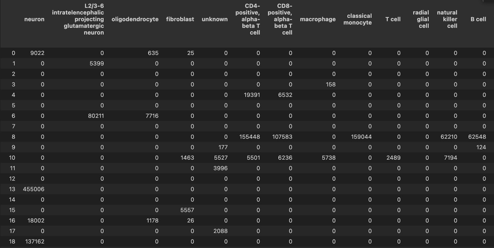
In order to ensure that we can test GenePT / scGPT hybrid models safely using the same test sets, we only include cells collected after the training date of scGPT (2023-05-08). In order to get good coverage in our test set we select the 20 files created after 2023-05-08 with the greatest number of different cell types. Note that this means that we might get cell types in our test set that do not appear in the training set.

This is another simple ILP, and so we can use the PuLP library to select our files.

Parameters:

Decision Variables:

$$x_i = \begin{cases} 1 & \text{if file is selected} \\ 0 & \text{otherwise} \end{cases}$$

Objective Function:

$$\min \sum_{i \in I} n_i \cdot x_i$$

Constraints:

$$\sum_{i \in I} c_{i,j} \cdot x_i \geq T \quad \forall j \in C$$

Optimizing this, we get 15 out of the 100 files that we can use for quick monitoring. This optimization takes 1.6 seconds on my laptop. Naively trying all possible subsets would require

$$2^{100} \approx 1.2e30$$

comparisons, or if we limit ourselves to “only” subsets of size 20 or fewer, then

$${100 \choose 20} \approx 5.4e20$$

Nice improvement!

A few years ago, I probably would have just chosen a few files at random instead of doing this optimization. A naive brute force approach would probably be more complex to implement, would probably be quite slow, and getting up to speed on a new library like PuLP would take more time that it is worth for a monitoring data set. An LLM makes this kind of code easy to get working very quickly, and improves the quality of my work for very little effort!

We then select up to 2000 cells of each type, for a total of 120,984 cells to make up our test set. This is our validation set that we will use to track the progress of training runs and compare different models.

We also want a smaller set for finer grained monitoring of the training dynamics. 5000 cells is probably enough to get a good directional read on the training process, so we create a balanced 5000 cell set by dividing 5000 by the number of cell types in the test set, and take that many of each type, filling in with other types when we don’t have 5000/|C| cells of a give type.

Next up: build a classifier that actually works

In training our classifier, we abandon XGBoost and gradient boosted trees because of the constraints they put on scaling, and confront a new set of challenges around distribution shift between batches. We also experiment with different metrics for measuring our performance, and visualize our cell type probabilities using a confusion matrix-ish heatmap.

Stay tuned! As always, your questions and feedback, especially negative, is greatly appreciated. Find me on

Lab Notes: Building a GenePT Cell Typer - Part 2