Objective

To explore Partial Dependence (PD) and run it in R script. This article is based on information in 「機械学習を解釈する技術 ~Techniques for Interpreting Machine Learning~」by Mitsunosuke Morishita. In this book, the author does not go through all the methods by R, so I decided to make a brief note with an R script.

Partial Dependence

Partial Dependence (PD) is a method to show the dependence between the response variable and explanatory variable. By changing the value of the explanatory variable while keeping track of the prediction, we can understand the relationship between the explanatory variable and the response variable. For example, if we increase the unit of explanatory variable $X0$, and the response variable also increases, these variables have a positive relationship. In addition to that, by potting these outputs, we can determine whether these variables have a linear or non-linear relationship.

Formula for PD

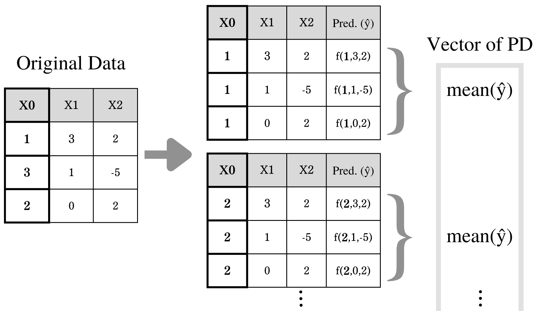
Here comes your favorite part. Based on the image above, let's say your trained model $\hat{f}(X0,X1,X2)$ and you would like to find out PD of $X0$ and prediction $\hat{y}$. In this situation, we only change the value of $X0$ and average out the prediction.

$$ \\large \\hat{PD\_0}(x\_0) = \\displaystyle \\frac{1}{N} \\sum\_{i = 1}^{N} \\hat{f}(x\_0,x\_{i,1},x\_{i,2}) $$

We use $x$ to express direct specification.

For example, If we specify $X0$ to be 1, we substitute $x_0$ to 1. So the function is going to be look like

$$ \\hat{PD\_0}(1) = \\displaystyle \\frac{1}{N} \\sum\_{i = 1}^{N} \\hat{f}(1,X\_{i,1},X\_{i,2}) $$

Or if we specify $X04$ to be 4, then

$$ \\hat{PD\_0}(4) = \\displaystyle \\frac{1}{N} \\sum\_{i = 1}^{N} \\hat{f}(4,X\_{i,1},X\_{i,2}) $$

$x_{i,1}$ and x_{i,2} takes $i$th observation of $X1$ and $X2$.

Or if you generalize more, define your set of explanatory variable as $X = (X_0,...,X_J)$, and define your trained model as $\hat{f}(X)$. Your target explanatory variable is $X_j$, and $X$ without $X_j$ is $X_{-j} = (X_0,...,X_{j-1},X_{j+1},...,X_J)$. Actual observation of $X_j$ at $i$th observation is defined as $x_{j,i}$. So actual observation without $x_{j,i}$ is x_{i,-j} = (x_{i,0},...,x_{i,j-1},x_{i,j+1},...,x_{i,J}).

When explanatory variable $X_j = x_j$, $\hat{PD_j}(x_j)$ aka. prediction mean is

$$ \\large \\hat{PD\_j}(x\_j) = \\displaystyle \\frac{1}{N} \\sum\_{i = 1}^{N} \\hat{f}(x\_j,x\_{i,-j}) $$

A method like this; calculating the effect of a focused variable by taking an average of other variables to ignore their effects, is called Marginalization. if you learn more about marginalization visit here

Execution with Real Data

Now, let's see how to run PD with actual dataset.

Get Dataset

# Set up
library(mlbench)
library(tidymodels)
library(DALEX)
library(ranger)
library(Rcpp)
library(corrplot)
library(ggplot2)
library(gridExtra)

data("BostonHousing")
df = BostonHousing

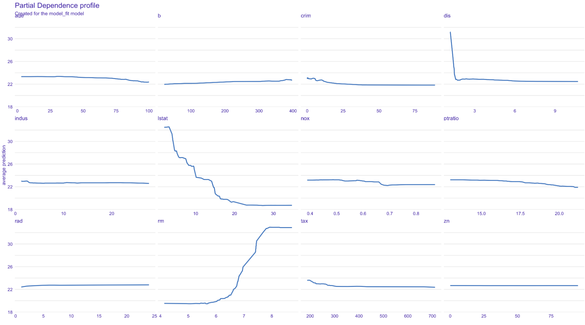
Obserview of the Dataset

Here are overview of the dataset

Build a Model

We won't cover building a model in this article. I used XGBoost model.

split = initial_split(df, 0.8)
train = training(split)
test = testing(split)

model = rand_forest(trees = 100, min_n = 1, mtry = 13) %>%
  set_engine(engine = "ranger", seed(25)) %>%
  set_mode("regression")

fit = model %>%
  fit(medv ~., data=train)
fit

Predict medv

result = test %>%
  select(medv) %>%
  bind_cols(predict(fit, test))

metrics = metric_set(rmse, rsq)

result %>%
  metrics(medv, .pred)

Interpre PD

Use the function explain to create an explainer object that helps us to interpret the model.

explainer = fit %>%
  explain(
    data = test %>% select(-medv),
    y = test$medv
  )

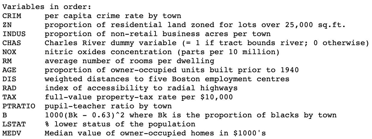
Use model_profile function to get PD plot. Here you can see lstat, rm, and dis (top 3 importance predictors by PFI) have relationships with prediction. The source code of model_profile is here.

pd = explainer %>%
  model_profile()
plot(pd)

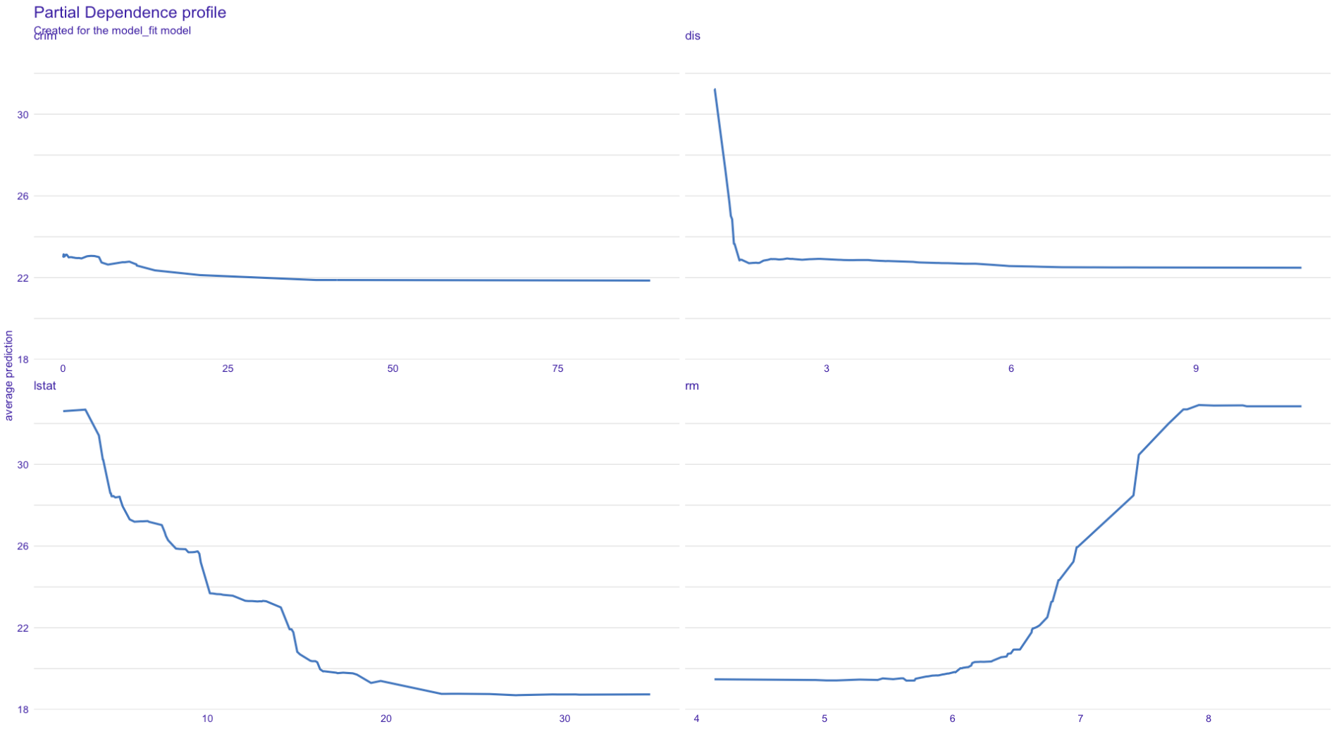
You can designate which plot you like to plot by giving variables method a vector of variable names.

pd = explainer %>%
  model_profile(
    variables = c("lstat", "rm", "dis", "crim")
  )
plot(pd)

FYI

Method	Function
Permutation Feature Importance(PFI)	model_parts()
Partial Dependence(PD)	model_profile()
Individual Conditional Expectation(ICE)	predict_profile()
SHAP	predict_parts()

dis, crim, and medv

Scatter Plot for All Variables

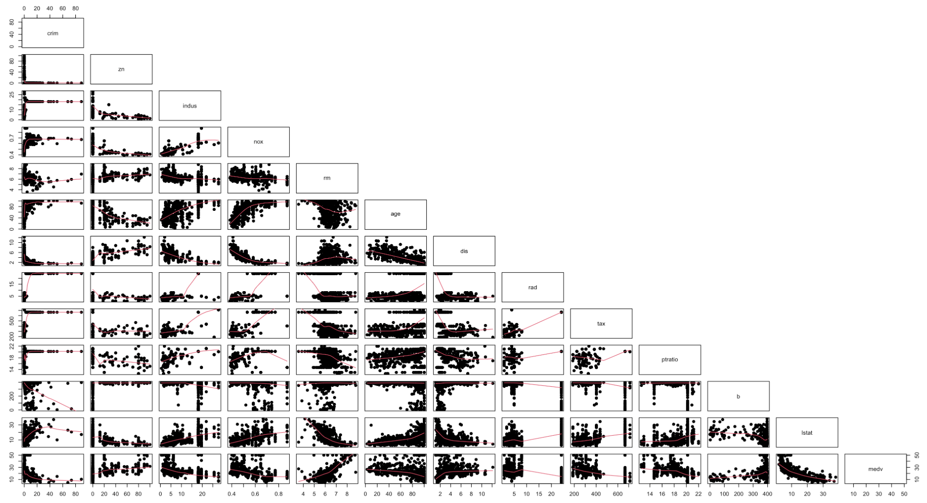
Some of you might ask, if the process of PD would be the same thing as just looking at the scatter plot like this. However, there is a huge difference between the scatter plot and the PD plot. First, look that the all scatter plots.

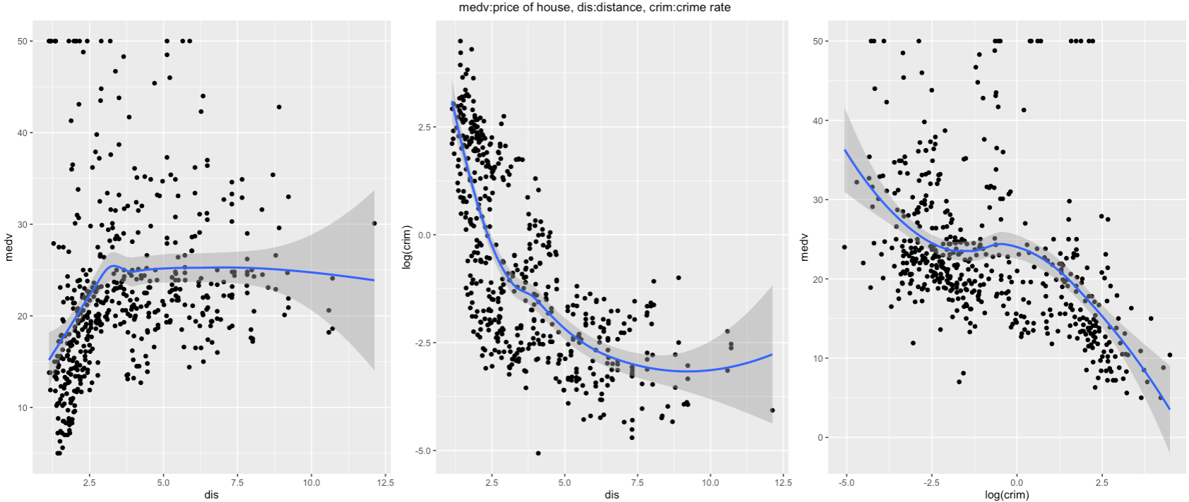
For example, take a look at the scatter plot above (dis; weighted distances to five Boston employment centers, crim; per capita crime rate by town, and medv; median value of owner-occupied homes in $ 1000's). Looking at the plot on the right, we can observe as the distance of employment centers and medv; median value of owner-occupied homes in \$1000's have a positive relationship. Since employment centers are located in the center of the cities, we can assume that as you move far from the city, the home price would increase. This is not very intuitive. By looking at crim and dis (the middle plot), the distance increases, crime rate decreases. From this observation, In Boston, the neighbor gets safer as you move away from the city center. Therefore, in the third plot, the price of the house decreases as the crime rate decreases. This explains the positive relationship between the home price and distance from the center.

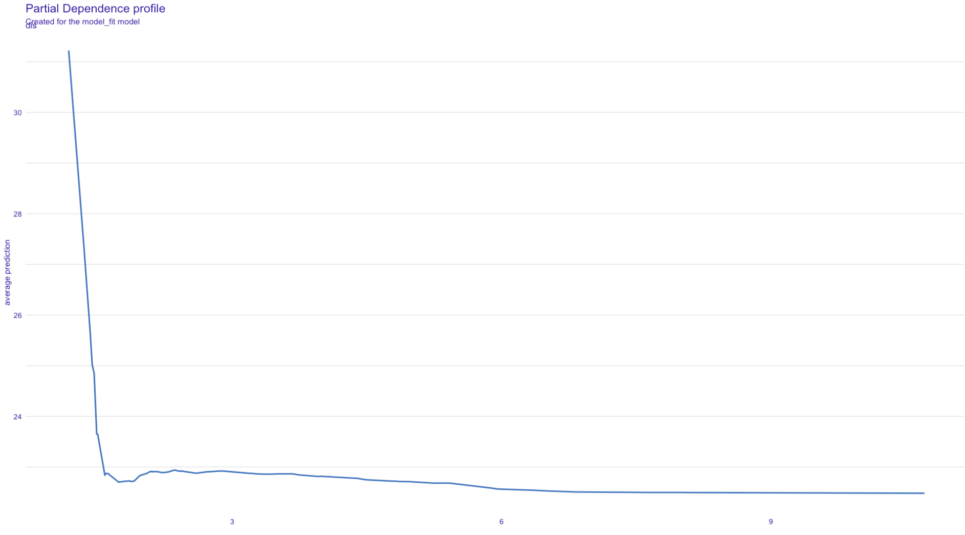
In PD plot, medv(y) and dis(x) have an opposite relationship to the scatterplot plot. As you can see, PD plot explains the hidden relationship between variables.

Conclution

PFI is the way to visualize the importance of explanatory variable. For deeper variable analysis, PD is a sufficient method to observe variable relationships. However, PD is averaging out all observations to visualize the relationship. If individual observations have different effects on the response variable, PD would not be able to catch that effects. in a situation like that, Individual Conditional Expectation (ICE) is capable of handling these effects.