Log #4: CNN Visualizer – Part 4
 John Boamah
Learning Objectives
By the end of Log #4, you will be able to:
Understand the fundamental problem that ResNet architectures solve
Explain the concepts of residual and skip connections
Analyze the architectural differences between ResNet18 and ResNet50
Interpret ResNet architecture diagrams and layer compositions
Decide when to use ResNet18 versus ResNet50 for different projects
Introduction
In this log, we were supposed to build the image upload endpoint, prediction endpoints, and integrate proper error handling and validation. But before diving into implementation, we need to understand the models we are working with: ResNet18 and ResNet50.
Deep neural networks (DNNs) have revolutionized computer vision, but training very deep networks introduces major challenges. One of these challenges was addressed by Residual Networks (ResNets), introduced by Kaiming He and colleagues in 2015. Before ResNets, deeper networks often performed worse than shallow ones due to the vanishing gradient problem and degradation issues. ResNet introduced the groundbreaking idea of residual learning. Instead of learning the desired underlying mapping H(x) directly, ResNet learns a residual function: F(x) = H(x) - x. This makes optimization easier and allows training of networks with hundreds or even thousands of layers.
The Residual Learning Concept
The core innovation of ResNet lies in its skip (or shortcut) connections. These allow the input to bypass one or more layers and are added directly to their output. Figure 1 shows a simple diagram of a ResNet
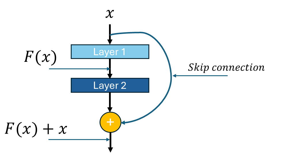
Figure 1: Simple Residual Network
Mathematically:
Traditional network:
H(x) = F(x)ResNet block:
H(x) = F(x) + x
Why skip connections matter
Gradient flow: Gradients can flow directly through skip connections, mitigating the vanishing gradient problem
Identity mapping: If the optimal function is close to identity, it’s easier to learn (F(x) = 0) than (H(x) = x)
Deep training: Enables effective training of much deeper networks
ResNet Building Blocks
ResNet uses two main types of residual blocks:
Basic Block (used in ResNet18)

Figure 2: Architecture of a basic block
Bottleneck Block (used in ResNet50)

Figure 3: Architecture of a bottleneck block
ResNet18 Architecture
ResNet18 is a relatively lightweight variant with 18 layers, making it suitable for scenarios with limited computational resources while still providing excellent performance.
ResNet18 Specifications
Total Layers: 18 (16 convolutional + 1 initial conv + 1 FC)
Parameters: ~11.7 million
Block Type: Basic blocks
Blocks per Stage: [2, 2, 2, 2]
Feature Maps: [64, 128, 256, 512]
ResNet50 Architecture
ResNet50 is deeper and more powerful, using bottleneck blocks to balance computational cost with model capacity.
ResNet50 Specifications:
Total Layers: 50 (49 convolutional + 1 FC)
Parameters: ~25.6 million
Block Type: Bottleneck blocks
Blocks per Stage: [3, 4, 6, 3]
Feature Maps: [256, 512, 1024, 2048]
Key Architectural Differences
| Aspect | ResNet18 | ResNet50 |
| Depth | 18 layers | 50 layers |
| Block Type | Basic Block | Bottleneck Block |
| Parameters | ~11.7M | ~25.6M |
| Computational Cost | Lower | Higher |
| Accuracy | Good | Better |
| Training Time | Faster | Slower |
| Memory Usage | Lower | Higher |
Skip Connection Variants
ResNet handles dimension mismatches in skip connections using two approaches:
Identity mapping: When input and output dimensions match
Projection shortcuts: When dimensions change (using 1×1 convolutions)
```python
# Pseudocode for skip connections
if input.shape == output.shape:
    return output + input  # Identity mapping
else:
    return output + conv1x1(input)  # Projection shortcut
```
Performance Characteristics
ResNet18 Use Cases:
Resource-constrained environments
Real-time applications
When training time is critical
Baseline experiments
ResNet50 Use Cases:
High-accuracy requirements
Transfer learning backbone
Feature extraction for complex tasks
When computational resources are available
Production systems prioritizing accuracy
Training Considerations
Batch Normalization: Critical for training deep ResNets effectively
Learning Rate Scheduling: Often use step decay or cosine annealing
Weight Initialization: Kaiming initialization works well
Next steps (Log#5)
In log#5, we will focus on creating the backend API endpoints for our CNN Visualizer, including:
Building an image upload endpoint to accept user images.
Adding an inference endpoint that runs predictions and returns activations.
Structuring JSON responses to be used on the frontend.
References
Goodfellow, I., Bengio, Y., and Courville, A. (2016). Deep Learning. The MIT Press, Cambridge, Massachusetts.
Simon J.D. P. (2024). Understanding deep learning.
Subscribe to my newsletter
Read articles from John Boamah directly inside your inbox. Subscribe to the newsletter, and don't miss out.
Written by